Thermomechanical

The thermomechanical analysis type uses Code_Aster to calculate the structural and thermal behavior of one or multiple bodies at once.

The thermal and structural result fields are calculated sequentially, in an iterative process, where the results of a thermal step serve as input for the next structural step. The stress state of the structure depends on the structural constraints and loads, as well as on the thermal expansion under thermal loads.

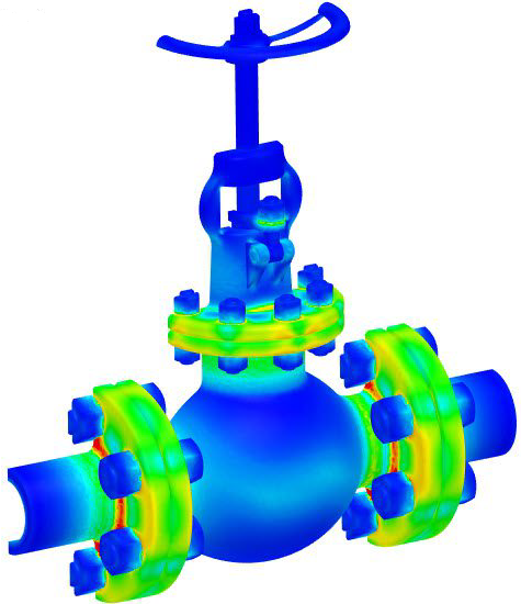
thermomechanical analysis type hot shock globe valve — Figure 1: Stresses on a globe valve due to a thermal shock

A thermomechanical analysis enables you to investigate the structural and thermal behavior of the model, as well as the thermal influences on the structural load state of the parts.

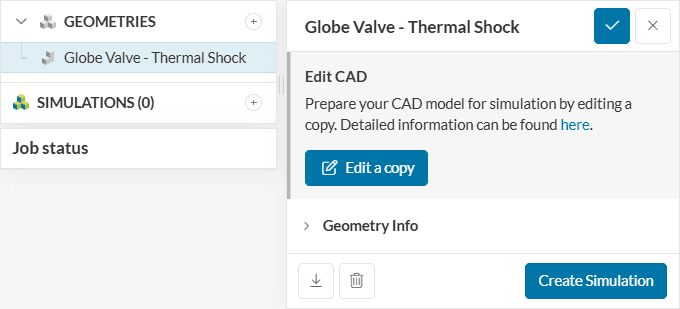
Creating a Thermomechanical Analysis

To create a thermomechanical analysis, select the desired geometry, and click on ‘Create Simulation‘:

new simulation run in simscale — Figure 2: Creating a new simulation in SimScale

The SimScale analysis type choice widget appears:

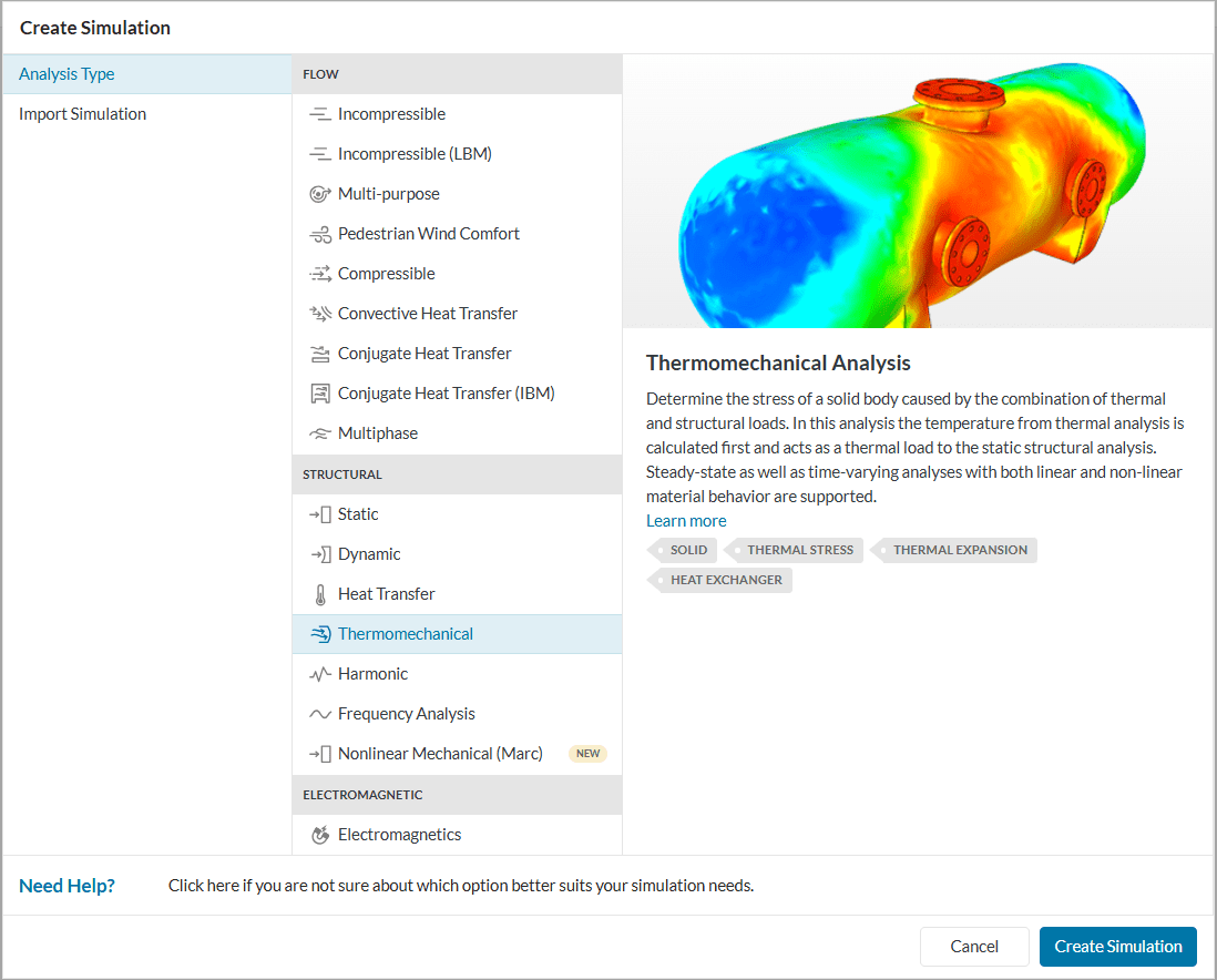
simscale analysis type choice widget with options — Figure 3: Creation of a new thermomechanical analysis

Choose ‘Thermomechanical‘ from the list and confirm your choice by clicking on the ‘Create Simulation‘ button. Figure 4 shows an overview of the settings available for a thermomechanical simulation:

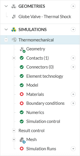
simulation tree thermomechanical analysis type — Figure 4: Simulation tree showing the entries for a transient nonlinear thermomechanical analysis

This document will describe the different simulation settings that need to be defined to run the simulation.

Global Settings

The global settings can be accessed by clicking on the simulation name, in this case, ‘Thermomechanical’ in the simulation tree. Here you can define the following:

Time dependency: the time dependency can be Steady state or Transient;
For transient analysis, users can also choose if the analysis will be Linear or Nonlinear.
Lastly, it’s possible to define the Inertia effects to Static or Dynamic. Inertia effects are only taken into account when Dynamic is selected.

For more information, check the global settings page.

Geometry

The Geometry tab contains the CAD model used for the simulation. Details of CAD handling are described in the pre-processing section. For more information on the CAD upload process and the subsequent steps please read our standard documentation.

Contacts

Assemblies of multiple bodies that are not fused, but touch each other, require contact definitions. All interfaces between bodies are automatically detected and defined as Bonded contacts when the simulation is created. Sliding contact and Cyclic symmetry contact definitions are also available.

For more information about contacts, have a look at this page.

Physical Contacts

The physical contacts tab will only be available in nonlinear analysis. There, users can define contact pairs of faces or face sets.

Physical contacts help to model contact behavior closer to reality. The distance between the contact faces is monitored during the simulation. If they touch each other, the interaction forces that prevent those faces from interpenetrating are taken into account.

Element Technology

Element technology refers to the numerical formulation for the solid finite element used in the simulation. This includes the mesh order, reduced integration, and mass lumping.

Model

In the Model section, one can define a gravitational load for the whole domain. Additionally, if your analysis is set to Nonlinear, you can determine the geometric behavior of the model.

Materials

A series of properties are defined under the Materials tab, including mechanical-related parameters, such as Young’s modulus and thermal-related parameters, such as the Thermal conductivity.

Furthermore, you can choose the material behavior describing the constitutive law that is used for the stress-strain relation.

Important

To define the material properties of the domain, make sure to assign exactly one material to each part. Please see the materials section for more details.

Initial Conditions

Defining initial conditions is only required in case of a Transient analysis. The initial conditions should be defined carefully since they determine the initial state of the domain before the loads and constraints are applied. Therefore, they will influence the solution of the simulation.

Depending on the Global settings configuration, the following parameters may be available for initialization:

Displacements
\((U)\) Velocity
\((a)\) Acceleration
\((\sigma)\) Stress
\((T)\) Temperature

Per default, the displacements, velocities, and accelerations are initialized with a zero magnitude vector. Temperature is initialized globally at 20°C. Additionally, when available, the initial stress state is taken as zero.

Users can change the initial settings of all five parameters, using global or subdomain initialization.

Boundary Conditions

In a thermomechanical analysis, one can define constraints, loads, thermal loads, and temperature boundary conditions.

Constraints and Loads

To determine the position of a part of the geometry, add at least one displacement constraint in every coordinate direction. Otherwise, the part is allowed to freely move in space. This is intended, for example, in drop tests.

In case no force boundary conditions are defined (including gravitational force), the geometry becomes load-free. In this case, apart from the prescribed displacement boundary conditions, no deformation will evolve. This might be intended to determine the strain distribution, for example, in pre-clamped structural components.

Temperature and Heat Flux

You can define temperature and thermal load boundary conditions. If you provide a temperature boundary condition on an entity, the temperature value of all contained nodes is set to the given prescribed value.

Thermal load boundary conditions define the heat flux into or out of the domain via different mechanisms. Note that a negative heat flux indicates a heat loss to the environment.

Important

It is not possible to simultaneously prescribe a temperature value and a thermal load to the same entity. This results in an overconstrained boundary.

This documentation page contains a list of all boundary conditions with additional information.

Numerics

Under numerics, you can set the equation solver of your simulation. The choice highly influences the computational time and the required memory size of the simulation. For an overview of the solvers available, please check this page.

Simulation Control

The simulation control settings define the overall process of the calculation. There you can set, for example, the time step length and the maximum runtime for your simulation.

Result Control

Under Result control, users can specify additional parameters of interest to be calculated. Monitors can also be defined. For example, one can set area and volume average controls, as well as Point data for monitoring quantities on specific points.

Please refer to the result control page for further insight.

Mesh

Meshing is the discretization of the simulation domain. It essentially means to split up one large problem into multiple smaller mathematical problems.

For a thermomechanical analysis, the standard algorithm is available. The standard mesher is recommended, as it is more robust.