Documentation
Under Field calculations, the user can define a series of additional outputs for their simulations, including total pressure, vorticity, amongst others.
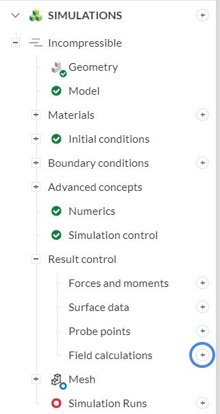
New field calculations can be defined under the Result control tab, as in Figure 1:
Important
If you are interested in one of the field calculation outputs, make sure to set it up before running the simulation.
Result controls are never applied retroactively to older simulation runs.
Below, we will go over each one of the Field calculation options available in SimScale.
The pressure field control is only available for the incompressible analysis type. With this field calculation, the user can define a series of different outputs, most notably Total pressure and Pressure coefficient, also known as \(C_p\). Find below some useful configurations.
For incompressible analysis, the default pressure values shown in the post-processor are gauge static pressures. If you are interested in having one additional scalar showing total pressures, this is also possible. Find below one sample result control configuration:
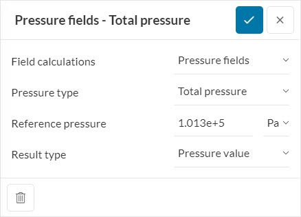
The platform will perform the following equation to show total pressure in the post-processor:
$$P_{Total} = P_{Gauge,\ static} + P_{Reference} + 0.5\rho U^2 \tag {1}$$
Where:
A result control for pressure coefficient can be created with the following configuration:
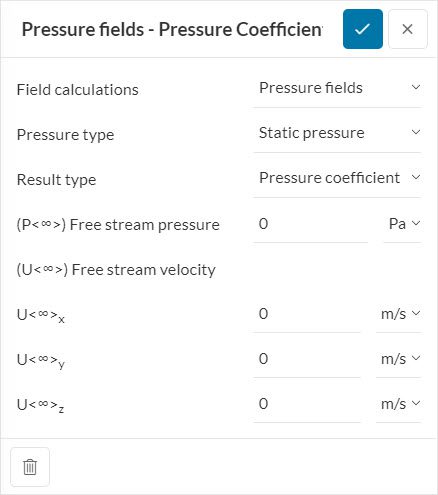
In Figure 3, the user should define their Free stream velocity based on the global coordinate system. Based on the input settings, SimScale uses the following formula to calculate the pressure coefficient \(C_p\):
$$C_p = \frac{P_{Gauge,\ static}\ – \ P_{Free\ stream}}{0.5\rho U^2} \tag {2}$$
Where:
The Turbulence result control allows the user to evaluate the yplus values in the post-processor. This parameter is very important for applications such as external aerodynamics and turbomachinery.
This result control is available for incompressible, compressible, and convective heat transfer analysis types. Note that the turbulence model must not be Laminar for the Turbulence result control to be available.
For background information on yplus and useful formulas, please check this post.
From a physical standpoint, one can understand vorticity as a vector having a magnitude equal to the maximum “circulation” at each point. Furthermore, the vector is oriented perpendicularly to the plane of circulation for each point1.
In the SimScale post-processor, vorticity is represented by vectors containing components in the x, y, and z directions, as well as a magnitude.
From a mathematical perspective, vorticity is defined as the curl of the velocity vector, as in Equation 3:
$$ Vorticity = \nabla \textrm{🗙} \vec{U} \tag{3}$$
Note
The vorticity result control is available for incompressible and incompressible (LBM) analysis types.
The mean age of fluid result control can be used to compute the local mean age of any fluid (ex: Air or Water) in the unit of seconds. This is nothing but the time a particle takes to travel from the inlet to the outlet.
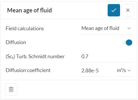
The diffusion term used to calculate the age of fluid can be enabled or disabled. When enabled, the Turbulent Schmidt number (\(Sc_{t}\)) and Diffusion coefficient \(D\) can be defined. The diffusion coefficient controls the laminar diffusion rate. For turbulent flows, the overall diffusion coefficient is calculated as:
$$\Gamma= D \rho + \frac{\mu_{eff}}{Sc_{t}} \tag{4} $$
Where \(\Gamma\) is the diffusion term, and \(\mu_{eff}\) is the effective viscosity.
Some commonly found diffusion coefficients are:
This result control is available for incompressible, convective heat transfer, and conjugate heat transfer simulations.
The Nominal turnover time \((\tau )\) given by\(^4\):
$$ \tau= \frac {V}{Q} \tag{5}$$
Where \(V\) is the volume of the test environment and \(Q\) is the volumetric flow rate at the inlet.
A perfect mixing situation occurs when there are no recirculation regions and the fluid is perfectly mixed within the test environment. In such a situation, we can say that
$$ Mean\ age\ of\ fluid = \tau = \frac {V}{Q} \tag{5}$$
The wall shear stress result control can be set in Incompressible, Compressible and Convective Heat Transfer simulations. As an output, the user obtains wall shear stress components in the x, y, and z-directions. Furthermore, the resultant vector for wall shear stress is also available.
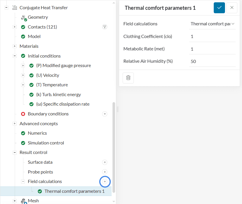
This result control complies with the methodology of both ASHRAE 55 and ISO 7730 Standards. By setting up a thermal comfort parameter under result control, the post-processor will contain two additional scalars:
A series of parameters may affect the PPD and PMV values, including the clothing coefficient, metabolic rate, and relative air humidity:
For more detailed insights about the set up of a thermal comfort parameter result control, please check this documentation page.
Note
The Thermal Comfort Parameters result control is available for convective heat transfer and conjugate heat transfer analysis types.
This field calculations result control item computes the friction velocity \(u_\tau\), which can be used to determine wall shear stress:
$$u_\tau = \sqrt\frac{\tau}{\rho} \tag {6}$$
Where \(\tau\) is the wall shear stress and \(\rho\) is the fluid density. Since both friction velocity and wall shear stress are vectors, we can rearrange equation 6 to account for the direction of the vectors when calculating wall shear stress:
$$\vec {\tau} = \rho\ mag\ (\vec{u_\tau})\vec{u_\tau} \tag{7}$$
Where \(mag\ (\vec{u_\tau})\) indicates the magnitude of the friction velocity vector.
Note
This result control is only available in the incompressible (LBM) analysis type. To calculate the wall shear stress field, it’s possible to take the SimScale results to ParaView and use the Calculator filter.
The surface normals result control is only available for the Incompressible (LBM) solver. This result control item is mostly used for further post-processing in third-party software, such as ParaView. The surface normals are not available for visualization in the SimScale post-processor.
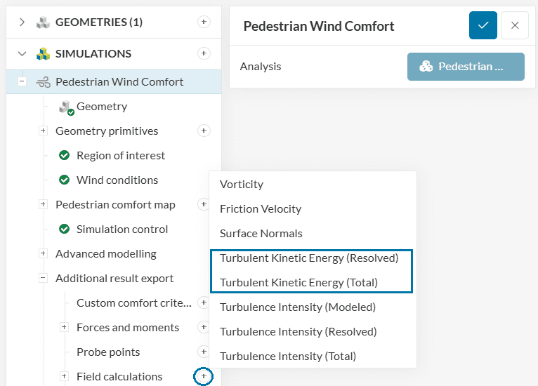
Turbulent Kinetic Energy and Turbulence Intensity fields are only available in PWC / LBM simulations. Most turbulence models don’t directly simulate all turbulence scales due to computational cost. Instead, they model the effects of the smaller, unresolved scales on the larger scales. This gives rise to two types of solutions namely, Modeled and Resolved. A combined result of both these solutions is then termed as Total.
The Turbulent Kinetic Energy (Modeled) is always calculated by the solver’s turbulence model as a default solution field and is therefore not available in the fields calculation menu but can be found in the post-processor. If none of the other TKE fields are added in the Result Control, this is simply named as Turbulent Kinetic Energy.
Turbulent Kinetic Energy (Resolved) is turbulent energy that is directly resolved and captured in simulation without any modeling. In LES, the large turbulent eddies are directly resolved by the simulation, and only the smaller, sub-grid scale turbulence is modeled.
Turbulent Kinetic Energy (Total) includes both modeled and resolved turbulence. This is the total energy in the turbulence, combining both the energy from the larger resolved eddies and the smaller, unresolved eddies that are modeled.
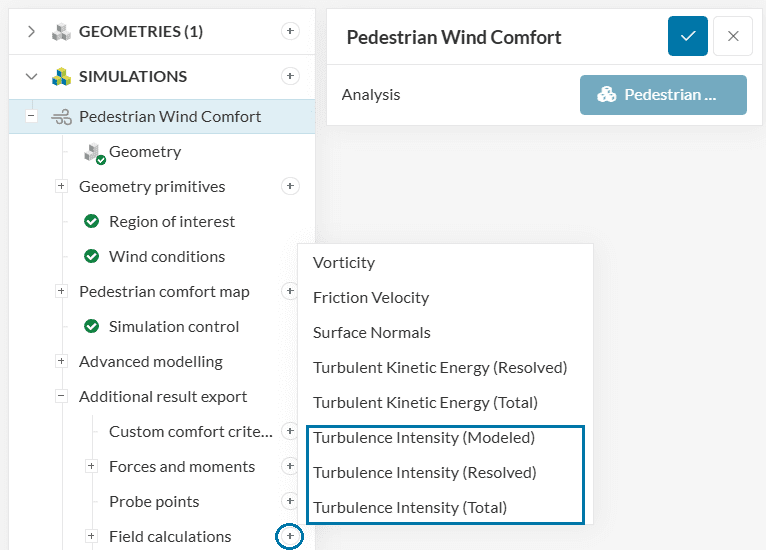
There are again three components to Turbulence Intensity similar to Turbulent Kinetic Energy:
The turbulence intensity gives the level of turbulence and can be defined as follows:
$$I = \frac { u’ }{ U }$$
where \(u’\) is the root-mean-square of the turbulent velocity fluctuations. Learn more.
Turbulence Intensity (Modeled) corresponds to the portion of the turbulence intensity that is modeled using a turbulence model, such as in RANS or the sub-grid scale (SGS) model in LES.
This turbulence intensity is associated with the resolved turbulent eddies, i.e., large-scale turbulent structures that are directly simulated.
The total turbulence intensity includes contributions from both the resolved and modeled components.
Note
New fields will be available under averaged results only and will not be available under transient field data for these additional result exports . Any added turbulent kinetic energy field will also be evaluated and exported by the Probe Point data.
This field calculation is available in Convective Heat Transfer, Conjugate Heat Transfer, Conjugate Heat Transfer (IBM) simulations. It retrieves the heat flux (units of power per surface area (\(W/m^2\))) at each interface and boundary wall of the model. Also, it has the option to automatically compute useful quantities that describe the heat transfer, such as the Heat transfer coefficient and the Nusselt Number:
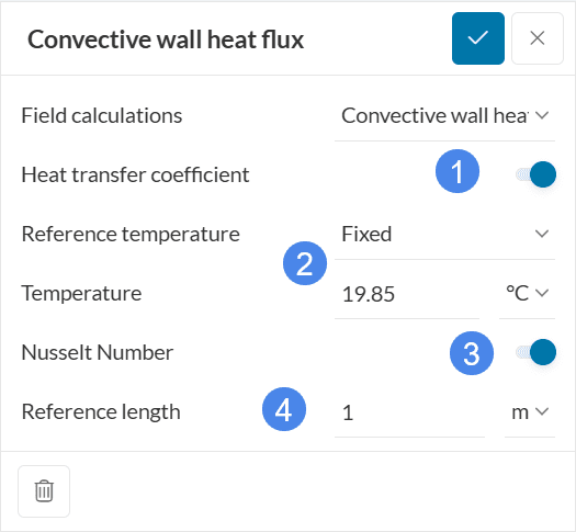
The heat transfer coefficient (\(h\)) appears in the convective heat transfer equation (Newton’s law of cooling), relating the heat flux (\(Q\)) and the temperature difference with the reference value (\(T_{ref}\)):
$$ Q = h A_s(T_s – T_{ref}) \tag{8}$$
The Nusselt number \(Nu\) can be related to the heat transfer coefficient \(h\), the reference length \(L\) and the thermal conductivity \(\kappa\):
$$ Nu = \frac{Convective Heat Transfer}{Conductive Heat Transfer} = \frac{ h L }{ \kappa} \tag{9}$$
Please notice that the Heat transfer coefficient and the Nusselt number are properties related to the heat transfer in the flow, and as such will only be computed for fluid regions, not for solid regions.
Wall heat flux and Radiation
The heat transfer due to radiation on interfaces and boundaries is not taken into account for the computation of the wall heat flux, as this only concerns the heat transfer with the flow, e.g., convection and conduction. Please bear this in mind when you perform energy balance calculations.
Mean Radiant Temperature (MRT) is a field calculation exclusively available in conjugate heat transfer simulations. When solar load is enabled, by creating a mean MRT result control, you have MRT as a field on the post-processor for all points within the flow region.
Note that by creating a thermal comfort parameters result control you are also going to get MRT fields in the post-processor. This is because the mean radiant temperature values are used for more precise PMV and PPD calculations, which are related to the thermal comfort parameter result control.
You will find more information involving mean radiant temperature, as well as equations, in this documentation page.
The operative temperature combines the air temperature with the mean radiant temperature to provide an overall measure of thermal comfort, with the formulation described here.
This result control is only available for conjugate heat transfer simulations.
References
Last updated: February 20th, 2026
We appreciate and value your feedback.
Sign up for SimScale
and start simulating now