In the Volume Load boundary condition, a distributed load per unit volume is applied on a body (or set of bodies). It is useful to model body loads, such as weight, inertial effects, centrifugal force, electromagnetic loads, and any load that is proportional to the volume (or mass) of the body.
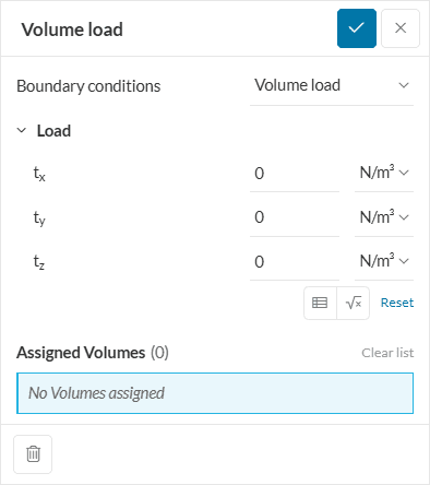
Figure 1: Volume load boundary condition panel. Enter the value in each direction with appropriate units and pick volumes to assign.
The parameters of the boundary condition are:
Load: The components of the applied load, expressed in the global coordinate system directions of the model ( (t_x, t_y, t_z) ).
Assignment: Set of volumes where the load will be applied.
Supported Analysis Types
The following analysis types support the usage of this boundary condition:
The traction vector is defined by the components of the load:
$$ vec{t} = (t_x, t_y, t_z) $$
Each component has units of force ((N), (lb.), etc) per unit of body volume ((m^3), (cubic in.), etc). The total applied force vector over the assignment set depends on the total volume:
$$ vec{F} = int vec{t} dV $$
Variable Load
Variable volume load values can be specified with the use of the formula or table inputs. The allowed functions are:
Time-dependent: The body force varies with respect to time (variable t) in a nonlinear static or dynamic simulation. This is useful, for instance, to ramp up the load from zero in nonlinear simulations, where a sudden application of load leads to numerical divergence, or for naturally time-varying loads in dynamic simulations.
Coordinate-dependent: The surface load varies with respect to the position in space (variables X, Y, Z). An example where this is useful is the case of hydrodynamic pressure, where the load varies with respect to the coordinates.
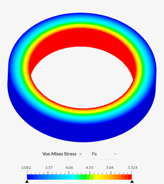
Figure 2: Stress contour plot of a ring subject to a centrifugal force, modeled with a volume load (see validation case below).