Tutorial: Incompressible Turbulent Airflow Around a Spoiler

This article provides a step-by-step tutorial for the flow simulation around a GT car rear spoiler using the incompressible turbulent flow analysis type.

Overview

This tutorial teaches how to:

• Set up and run an incompressible turbulent flow simulation.
• Assign boundary conditions, material, and other models to the simulation.
• Mesh the geometry with the SimScale standard meshing algorithm.

The typical SimScale workflow will be followed:

• Prepare the CAD model for the simulation.
• Set up the simulation.
• Set up the mesh.
• Run the simulation and analyze the results.

1. Prepare the CAD model and Select the Analysis Type

First of all, click the button below. It will copy the tutorial project containing the geometry into your own Workbench.

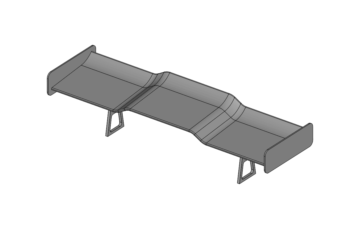
The following picture shows the geometry used for the simulation. It corresponds to a typical car spoiler, installed to increase the downforce in the rear axis:

1.1 Required CAD Preparation

You can see that there are two geometries in the imported project. The first one is called Original Spoiler and the second one is named Spoiler – Flow Region. The original model shows the geometry of the solid part to be analyzed:

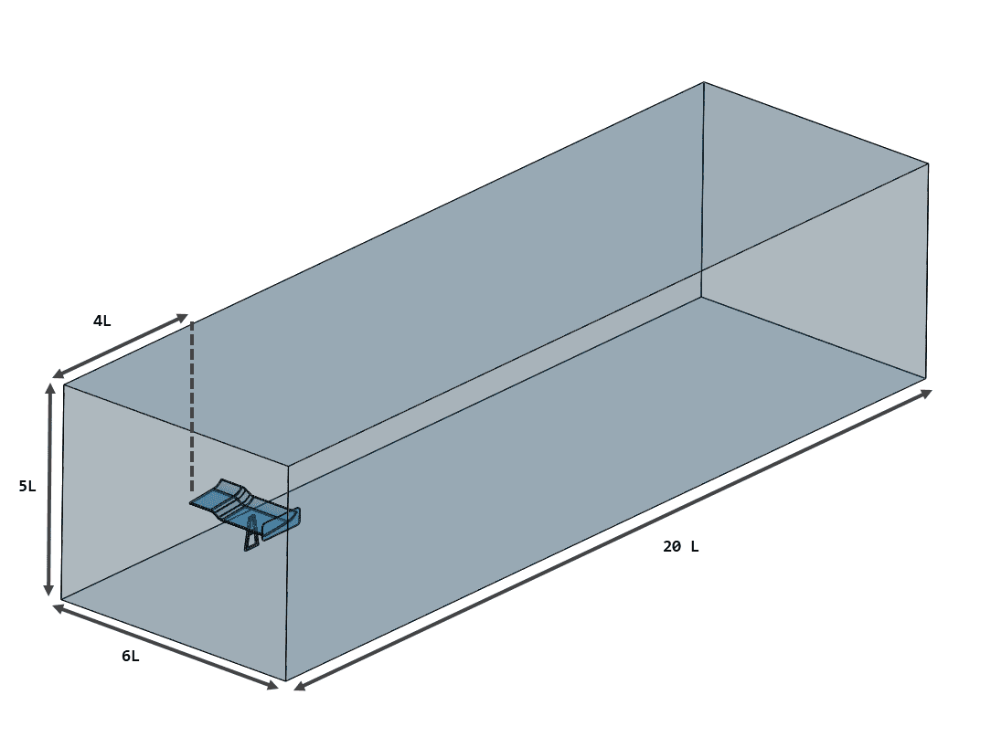
The Spoiler – Flow Region part contains the virtual wind tunnel representing the volume of air around the spoiler. Notice that, as the spoiler is symmetric, we simulate only one-half of the geometry to optimize simulation resources.

The image below shows how the bounding box dimensions were chosen, relative to the chord length of the spoiler, \(L = \) 0.25 \(m\).

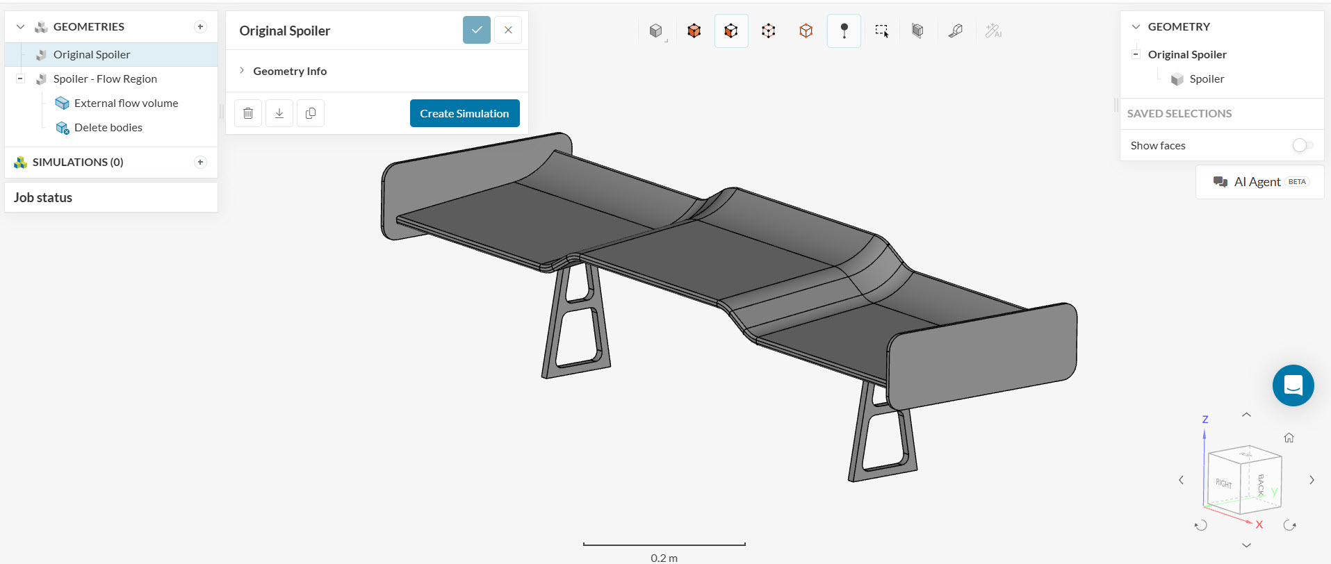
You can check the details of the flow volume creation by selecting the Spoiler – Flow Region geometrical object item on the left, and clicking the ‘CAD mode’ icon:

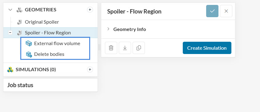
The CAD mode environment will open, with the performed operations shown under History:

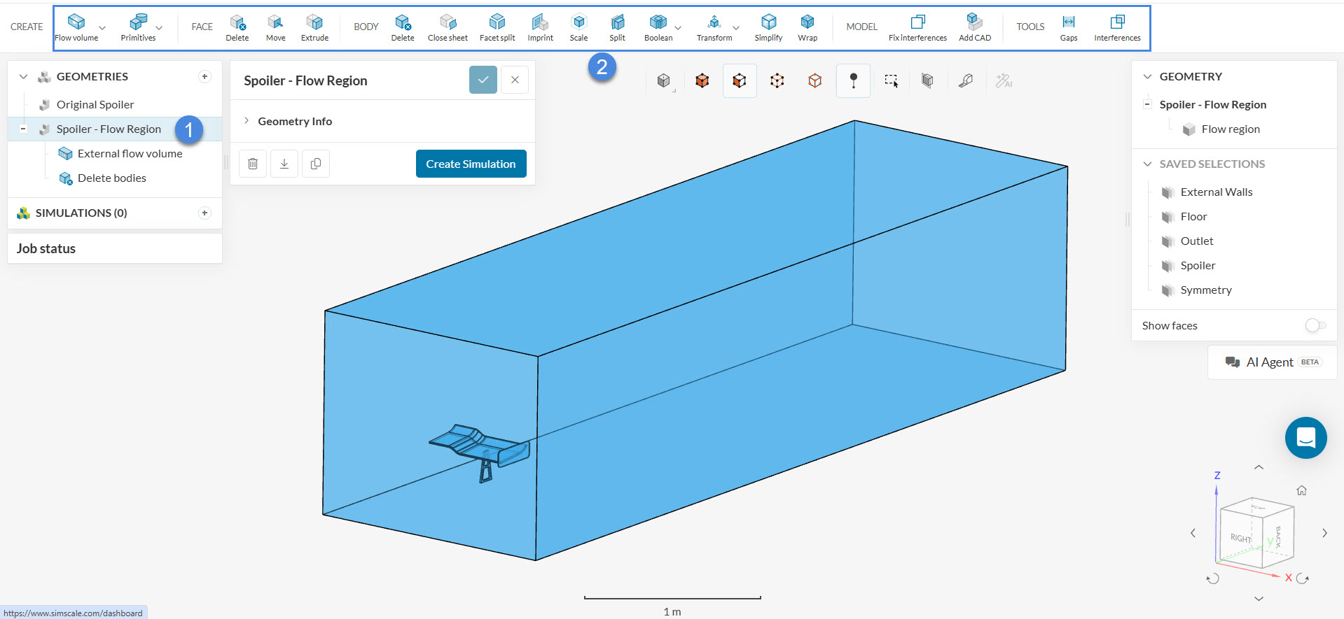
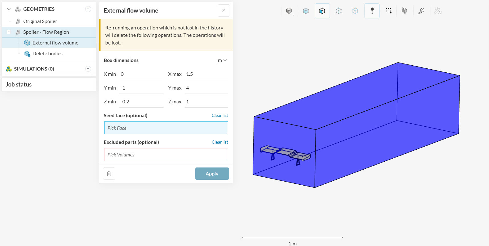
In CAD mode, two operations were performed:

1. External flow volume, to create the flow region (virtual wind tunnel), and
2. Delete bodies, to remove the spoiler part from the model

The details of the operations can be seen below:

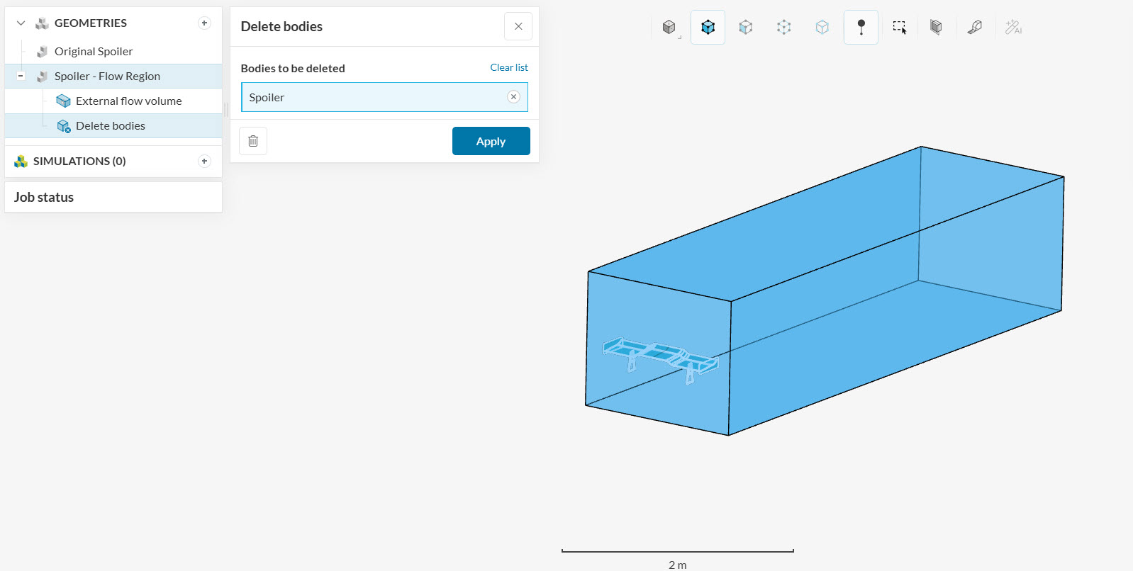
As this is an incompressible analysis, only the flow volume is necessary to run the simulation. Therefore, the spoiler volume is deleted with the operation below:

To exit from CAD mode, simply click on ‘Exit’ on the top-right corner.

1.2 Create Saved Selections

Saved selections are groups of faces used for boundary conditions or other assignments. By using them, the simulation setup can be done faster.

For the simulation setup, we will use the Spoiler – Flow Region geometry. After selecting the geometry, you will find pre-defined saved selections on the right-hand side panel:

Five of the needed sets are already provided in the template project, but the set for the flow inlet face is still missing. The picture below shows how to add it:

1. First, select the corresponding faces from the viewer (notice this is the one just in front of the spoiler).
2. Click the ‘+’ icon next to Saved Selections in the scene tree.

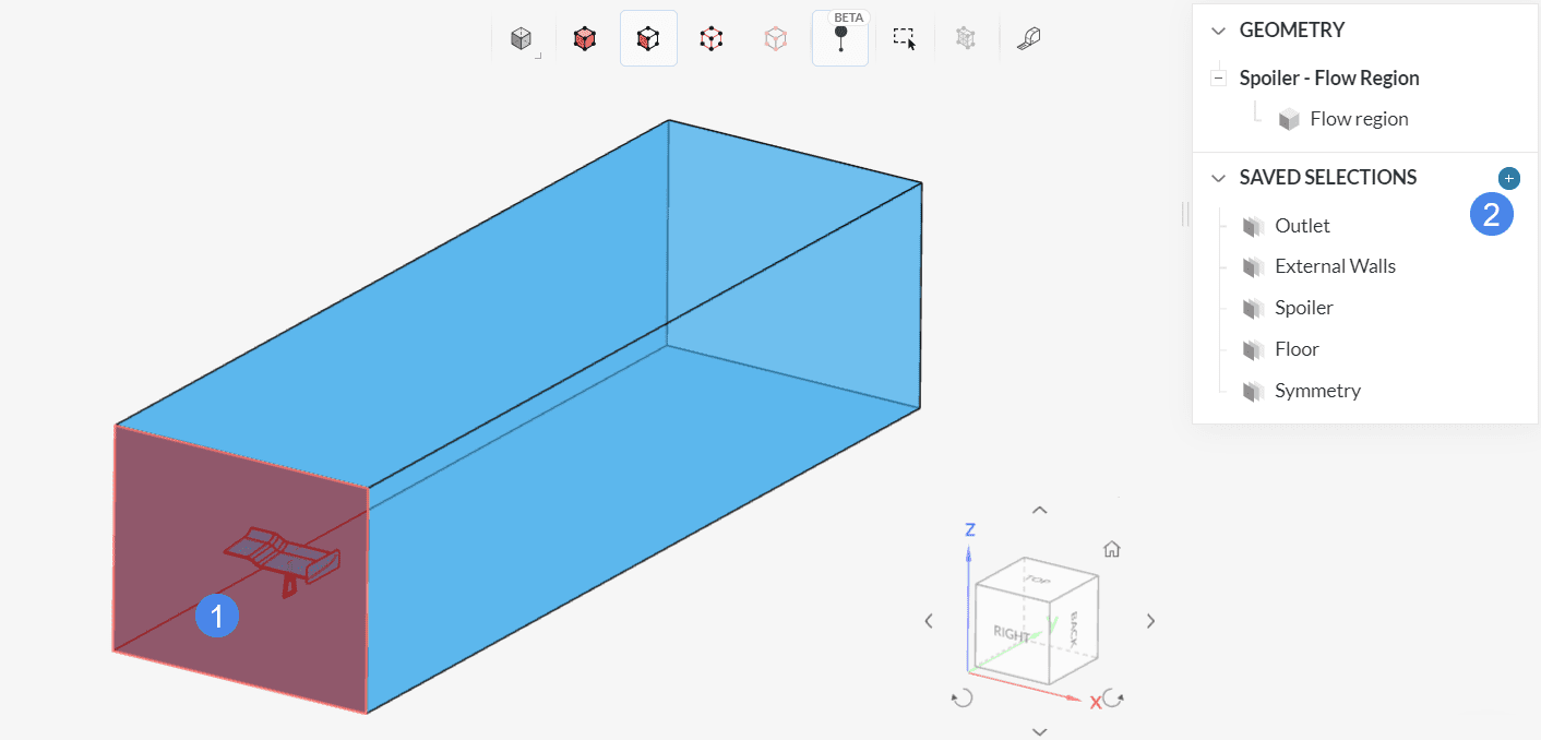
In the pop-up dialog that appears, name the set “Inlet” and click ‘Create new selection’.

1.3 Create the Simulation

Now we can start with the simulation setup. Follow the steps shown in Figure 6 and click the ‘Create Simulation’ button located at the bottom right of the panel. The simulation library window appears to select the appropriate simulation type:

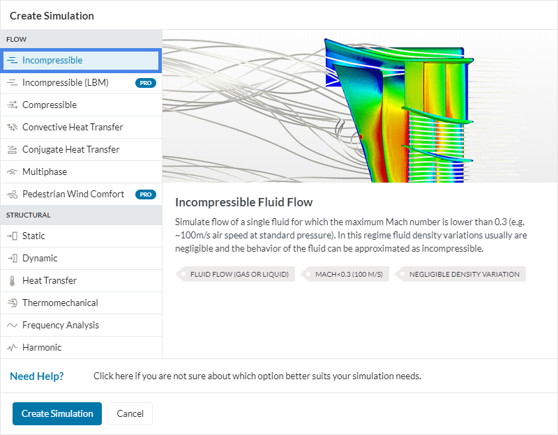
Choose ‘Incompressible’ and click on ‘Create Simulation’.

2. Set Up the Simulation

A new simulation tree will appear on the left-hand side of the Workbench. The first entry of the simulation tree is the global settings of the simulation. For this tutorial, please keep the default values:

From the Turbulence models available, this tutorial uses ‘k-omega SST’. For more details about its implementation, please check this page.

2.1 Material

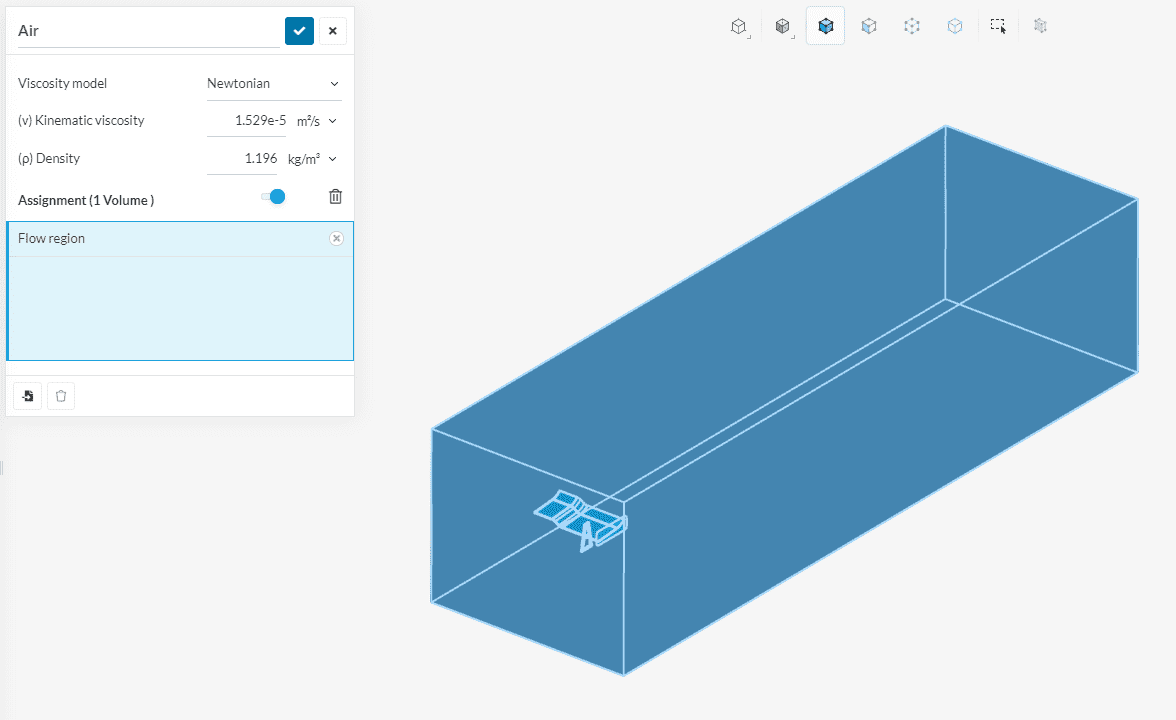
To define and assign a material, click the ‘+’ icon next to Materials. Doing so, the SimScale material library will pop up. Select Air from the materials library and click ‘Apply’:

The material properties window will appear. The Flow Region volume is automatically selected because it is the only one present in the model. Therefore, please accept the selection by clicking on the checkmark.

2.2 Boundary Conditions

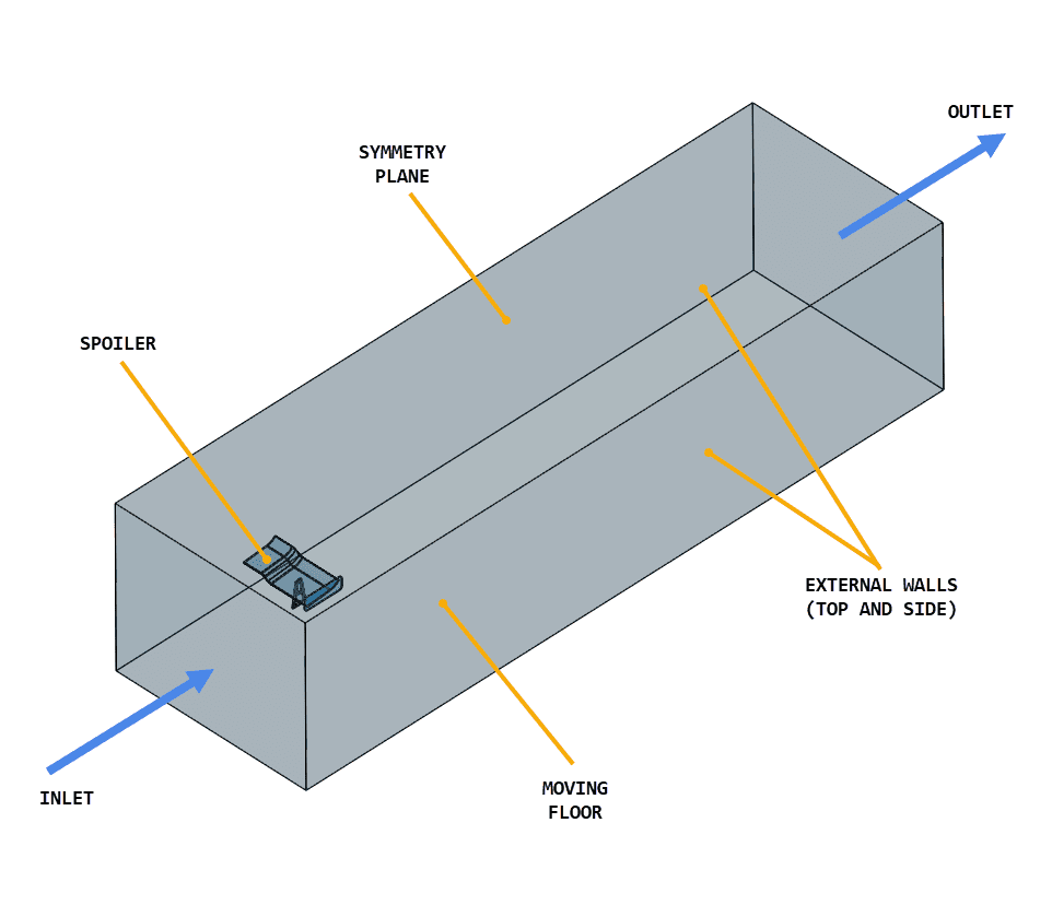
The image below contains an overview of the boundary conditions from this tutorial:

To create a boundary condition, follow the steps shown in the picture below:

1. Click the ‘+’ button next to Boundary Conditions.
2. Select the proper type from the drop-down menu.
3. Set up the physical parameters and assign faces in the pop-up dialog (not shown in the picture).

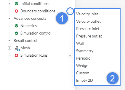
Now apply this process for the following boundary conditions:

a. Spoiler Surface

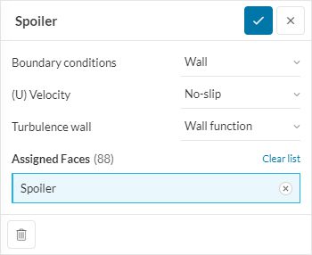
For the spoiler surfaces, a no-slip wall condition is used.

Following the instructions in Figure 18, select ‘Wall’. Now, select the Spoiler saved selections to assign it to the boundary condition – You can also rename the boundary condition to ‘Spoiler’.

Leave all parameters as default, as shown in the picture below:

b. External Walls

For the External Walls, please create another ‘Wall’ boundary condition. Once the setup panel pops up, select the ‘External Walls’ entity set that was created before for the assignment. The Velocity definition is Slip, allowing non-zero velocity in the tangent direction:

c. Inlet

For the flow inlet face, a velocity inlet boundary condition will be used. Follow the same procedure as before to create a ‘Velocity inlet’ boundary condition and assign the ‘Inlet’ entity set.

Set up the dialog as shown in the picture:

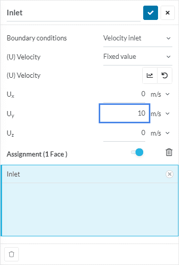
Define a fixed value velocity of ’10 \(m/s\)’ in the y-direction \((U_y)\).

d. Outlet

For the flow outlet face, a pressure outlet boundary condition will be used. Follow the same procedure as before to create a ‘Pressure outlet’ boundary condition and assign the ‘Outlet’ entity set.

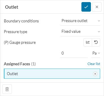
This tutorial uses the default settings for the pressure outlet condition.

e. Floor

For the floor below the spoiler, a moving wall boundary condition will be used. Create another ‘Wall’ boundary condition, and assign the ‘Floor’ entity set to it:

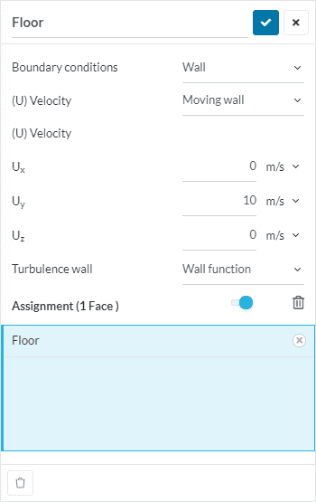
Select ‘Moving wall’ for (U) Velocity and assign ’10 \(m/s\)’ to the y-direction.

f. Symmetry

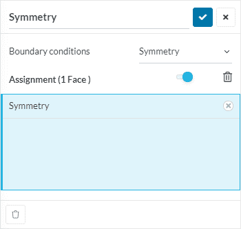
Finally, for the symmetry plane, create a ‘Symmetry’ boundary condition, assigning the ‘Symmetry’ saved selections.

Set up the parameters as shown in the picture below:

3. Simulation Control

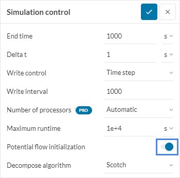
One important setup in order to help the simulation achieve good results and converge faster is the Potential flow initialization. Toggle it on inside the Simulation Control tab, as shown in the figure:

4. Mesh

For this tutorial, we are using the hex-dominant automatic mesher. Click on ‘Mesh’ from the simulation tree and define the global settings as follows. You can rename it as Hexahedral Mesh:

Do not generate the mesh just yet – click on the blue checkmark and save.

Before generating the mesh, we want to set a mesh refinement to capture the wake more accurately. Therefore we will create a region refinement:

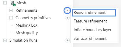
Click on the ‘+’ button next to Refinements and select ‘Region refinement’. This opens the settings panel.

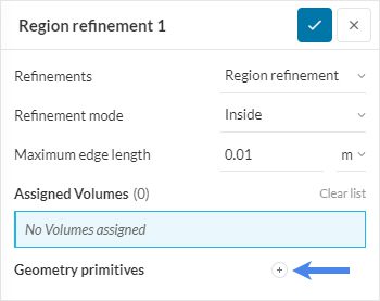
Set the Maximum edge length to ‘0.01 \(m\)’ and click on ‘+’ button to create a ‘Cartesian box’ geometry primitive for the volume assignment:

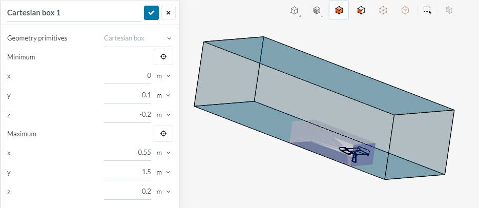
Define the following dimensions for the Cartesian box in meters as shown in the picture above.

• Minimum x: ‘0’ \(m\)
• Minimum y: ‘-0.1’ \(m\)
• Minimum z: ‘-0.2’ \(m\)
• Maximum x: ‘0.55’ \(m\)
• Maximum y: ‘1.5’ \(m\)
• Maximum z: ‘0.2’ \(m\)

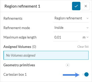
After saving the cartesian box settings, you are redirected to the region refinement settings. Assign the cartesian box that you just created. This ensures that all the cells within this box will have a maximum edge length of 0.01 \(m\).

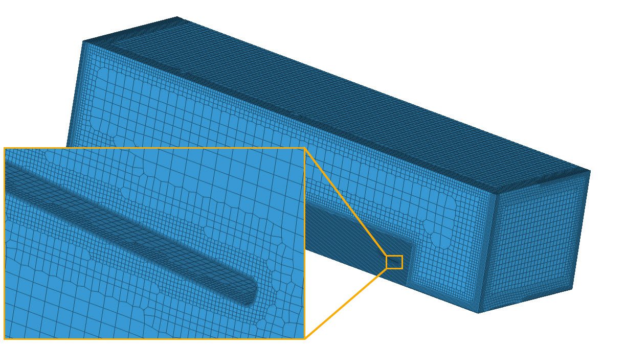
Save the settings and go back to the Mesh tab in the simulation tree and hit ‘Generate’ to create the mesh.

After around 30 to 40 minutes, you will see this mesh:

5. Start the Simulation

Now that the simulation setup is complete, a new simulation run can be created. For this, click the ‘+’ button next to Simulation Runs in the simulation tree. In the pop-up window, give a proper name to the run and click ‘Start’:

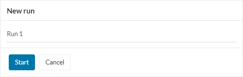
This computation takes about an hour. If you can’t wait to see the results, at the end of the article you will find a link to the completed version of the project.

6. Post-Processing

You can visualize your results by using SimScale’s online post-processor. We will visualize the pressure distribution on the spoiler, create a cutting plane, and animate the streamlines of the flow around the spoiler.

6.1 Pressure Distribution

One of the results of interest is the pressure distribution on the surface of the spoiler. Follow the steps below to visualize the same:

• When entering the post-processor for the first time, check if you are at the last time step of the simulation and there are no pre-defined filters. Also, change the Coloring of Parts Color to ‘Pressure’.

• The next step is to hide the enclosure. To do this, select the 6 external boundaries of the flow domain, and right-click on the viewer to ‘Hide the selection’:

• After hiding the enclosure, you will get a clear visualization of the pressure distribution on the spoiler similar to the figure below:

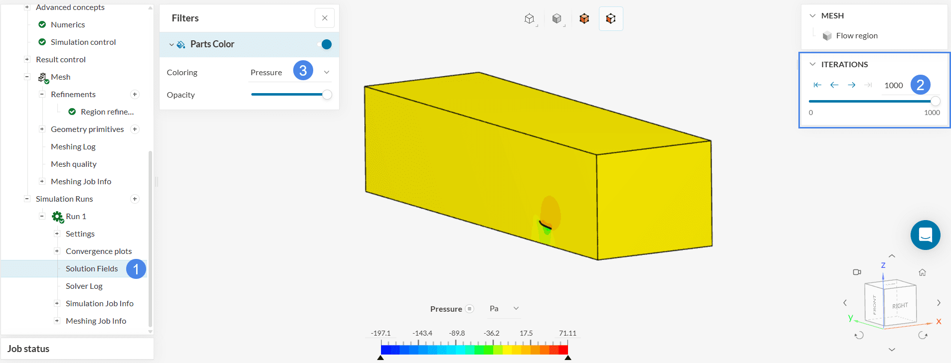
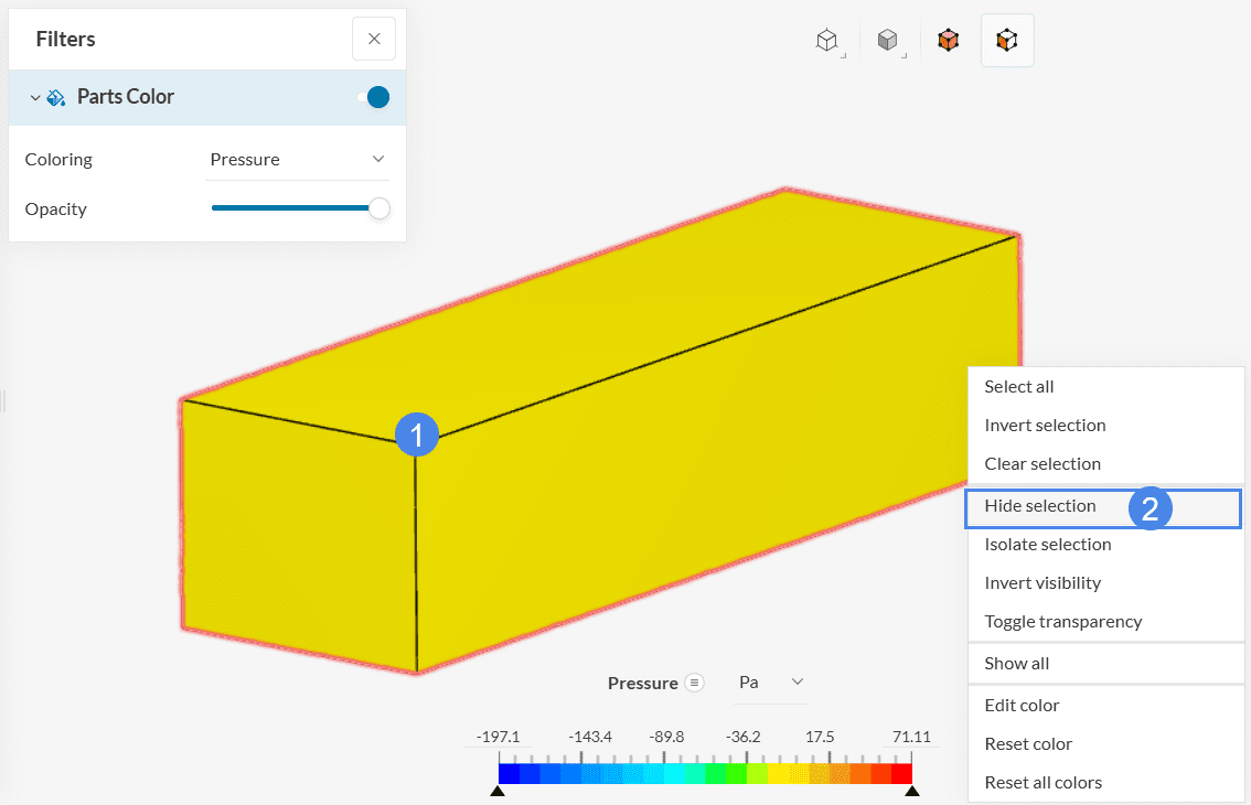
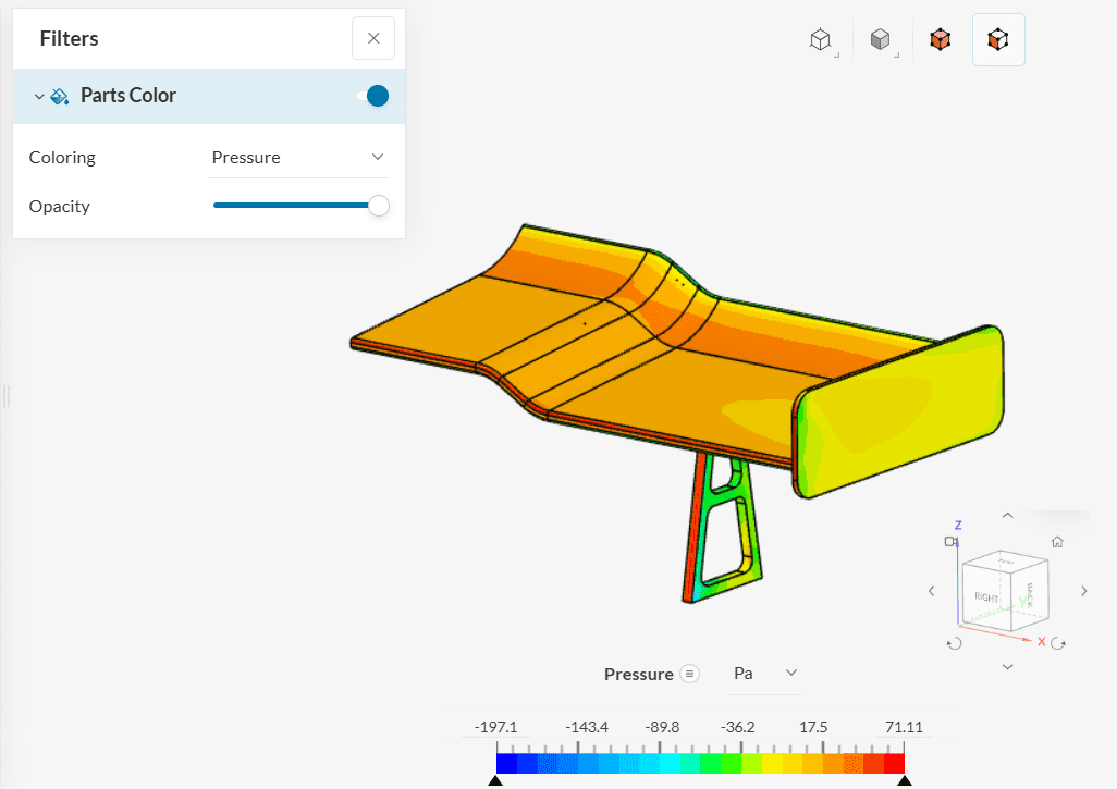
Figure 35 shows high-pressure contours on the top of the spoiler. Given the low-pressure regions under the spoiler, this combination results in downforce.

6.1 Cutting Planes

A cutting plane can also be used to better understand the turbulence around the spoiler and its characteristics. To create a cutting plane, select ‘Cutting plane’ from the Filters panel.

Next, place the cutting plane at the mid-section of the spoiler. Click on the arrow to the left of Position and set the values to ‘0.1, 1.5, 0.4’. Keep the Orientation normal to the ‘x-axis’. Switch Coloring to ‘Turbulent Kinetic Energy’. Finally, show the velocity vectors by sliding the toggle beside Vectors and changing the Coloring to black Solid color.

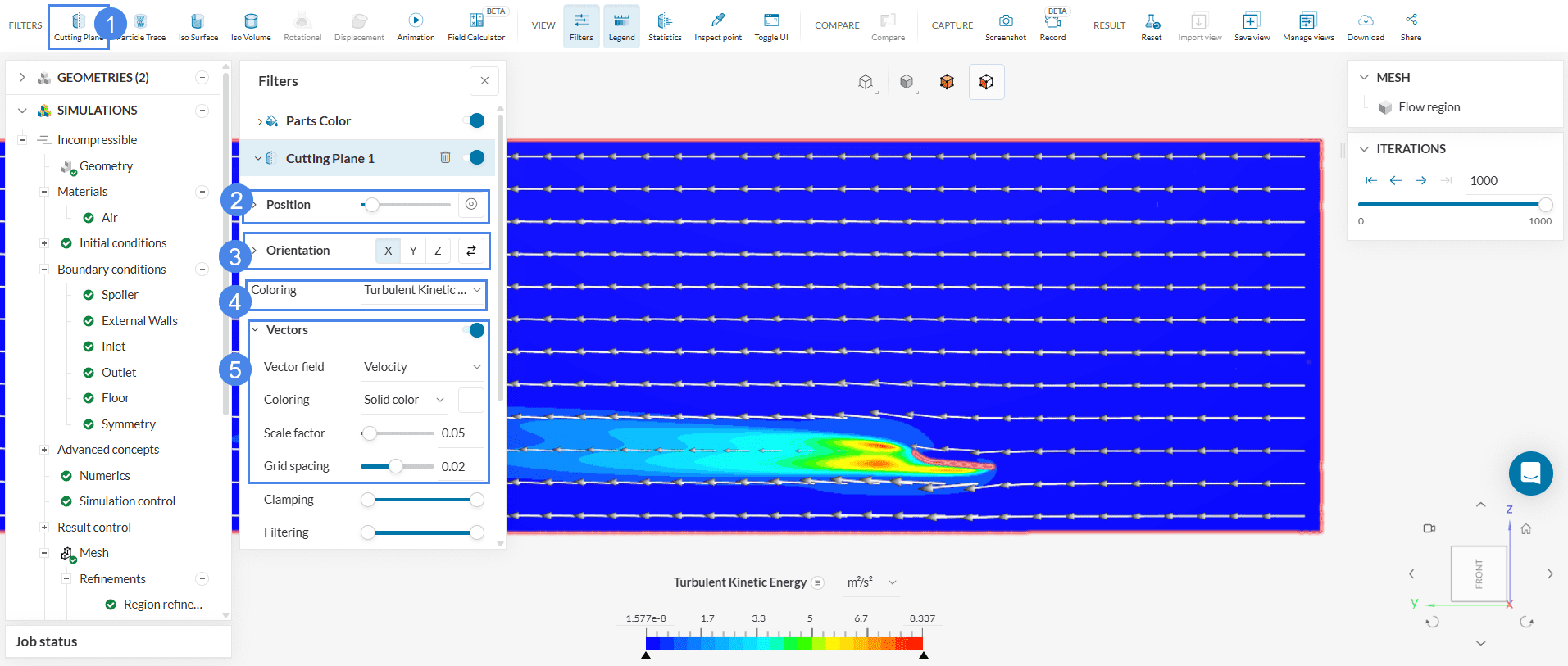
Here, we can see turbulence starts to occur when the flow hits the wing and is at its highest under and at the trailing edge of the wing.

6.3 Streamlines and Animation

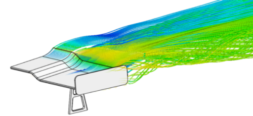
Another result of interest is visualizing the streamlines around the spoiler. Follow the steps below to show the streamlines and animate them:

1. From the top filters ribbon, choose ‘Particle Trace’
2. Make sure that the Pick Position selector is on
3. Choose a seed for the particle traces at the inlet, just in front of the spoiler

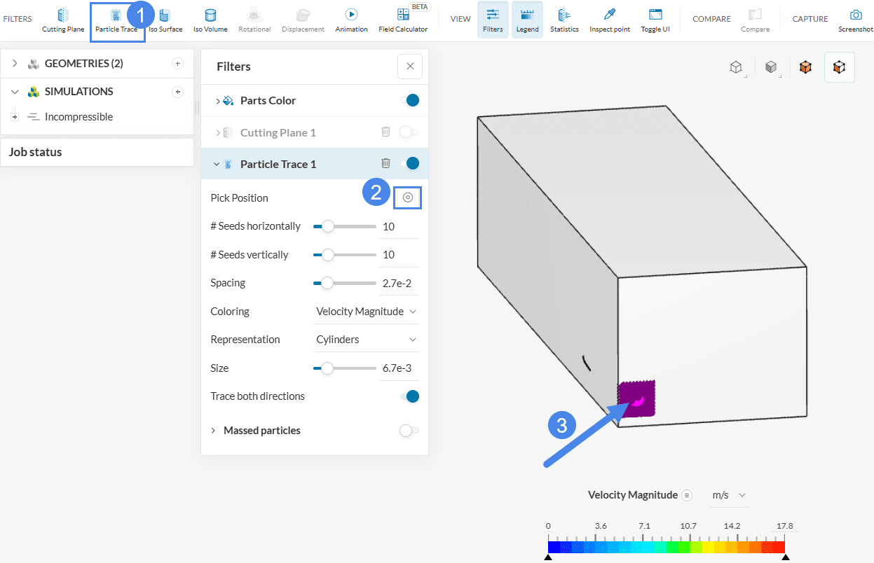
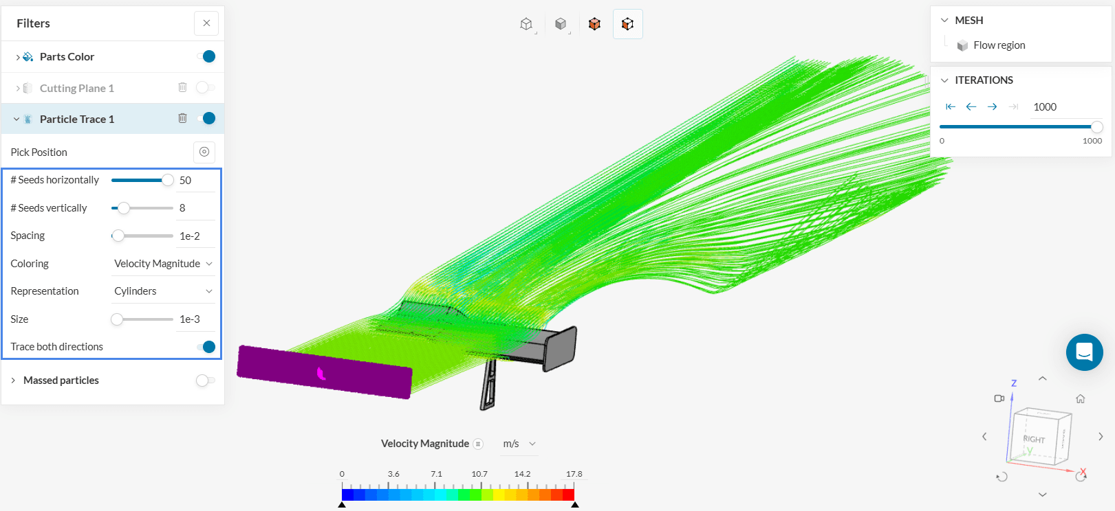
At this point, you can configure your particle traces so that the streamlines show relevant pictures. Change the number of particle traces by changing the values in #Seeds horizontally to ’50’ and #Seeds vertically to ‘8’. Change the Spacing to ‘1e-2’ and the Size to ‘1e-3’. Hide the walls of the fluid domain to see the streamlines around the spoiler. Finally, change the Coloring in Parts color to some contrasting white or grey solid color.

After creating the particle trace filter, it is possible to animate it with an Animation filter. Please use the filter ribbon on the top to create a new ‘Animation’ filter. The Animation type will be ‘Particle Trace’.

After the animation filter is set, you can press the play button to animate the traces:

Animation 1 displays the airflow streamlines. The generated tip vortices, the up-wash, and the low speed close to the surface (blue portions of the streamlines) can be appreciated from the images.

You can analyze your results with the SimScale post-processor. Have a look at our post-processing guide to learn how to use it.

Congratulations! You finished the tutorial!

Last updated: October 13th, 2023