Tutorial: Incompressible Flow around a Formula Student Car
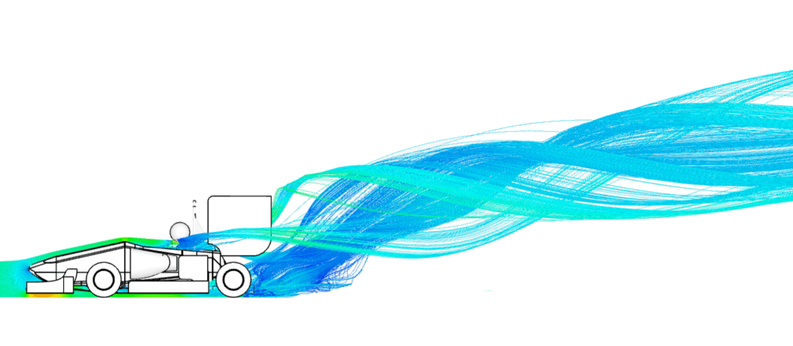
This tutorial shows how an incompressible turbulent airflow around a Formula Student car moving in a straight line can be simulated. Figure 1 shows an example of the resulting flow behavior:
This tutorial teaches how to:
- Set up and run an incompressible simulation;
- Use SimScale’s Edit CAD features;
- Assign saved selections;
- Assign boundary conditions, material, and other properties to the simulation;
- Mesh with SimScale’s standard meshing algorithm.
We are following the typical SimScale workflow:
- Prepare the CAD model for the simulation;
- Set up the simulation;
- Create the mesh;
- Run the simulation and analyze the results.
1. Prepare the CAD Model and Select the Analysis Type
Note, if you are not using the tutorial CAD model
Prepare the geometry for the simulation (only if you are not using the tutorial’s Edit CAD option):
- If the CAD model contains small features, fillets or round faces, which are unlikely to have an impact on the result, it is recommended to remove those details before importing the model into SimScale.
- Small and detailed features that don’t greatly affect the aerodynamics, such as bolts etc., should be removed or simplified.
- The solid volumes should be non-overlapping and should all be touching each other.
With this approach, you can reduce the computation effort necessary throughout the entire simulation process, while still obtaining meaningful results. Find more information about CAD preparation on this documentation page.
The first step is to click on the button below. It will copy the tutorial project containing the geometry into the Workbench.
The following picture demonstrates what should be visible after importing the tutorial project:
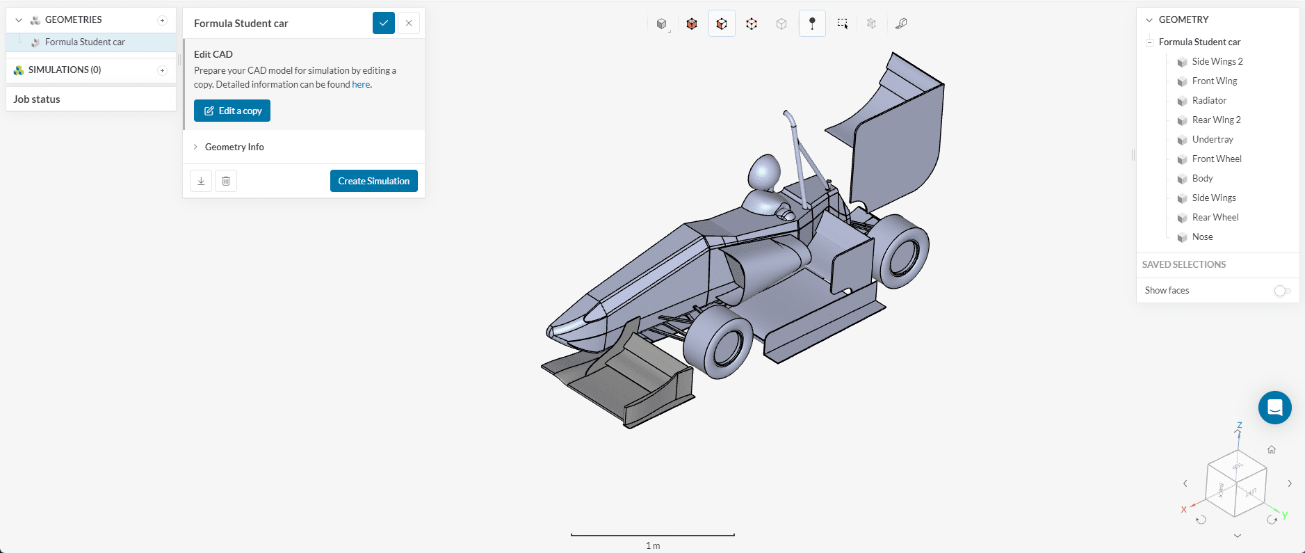
At the right of the Workbench, the parts of the model can be seen. This is a watertight assembly of the P19 model, provided by the Prom Racing FSAE Team, with an aerodynamic package of a rear wing, a front wing, a configuration of elements at the sides of the car, an undertray, and finally sidepods that enclose radiators. The suspension system can be included, as long as it is simplified.
1.1. Edit a Copy
For an incompressible analysis, only one part is allowed, which is the flow region. In case we want to add a cell zone too, we will have to include this part too. For the specific case, the car also includes a radiator, that will be modeled as a porous medium, so it is important that both the flow region and radiator remain as the only, and separate, parts. This is possible with the Edit CAD option feature that allows performing a variety of operations, such as flow volume extractions, parts deletion, etc.
Note
In case that the model does not include parts to be modeled as cell zones, you can create an Enclosure, as described in this documentation page.
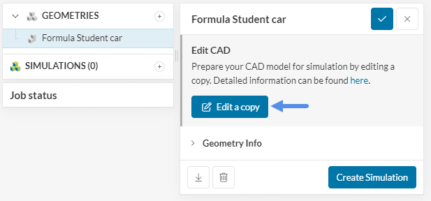
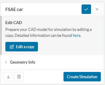
To enter the Edit the CAD, click on the Edit a copy as shown below:
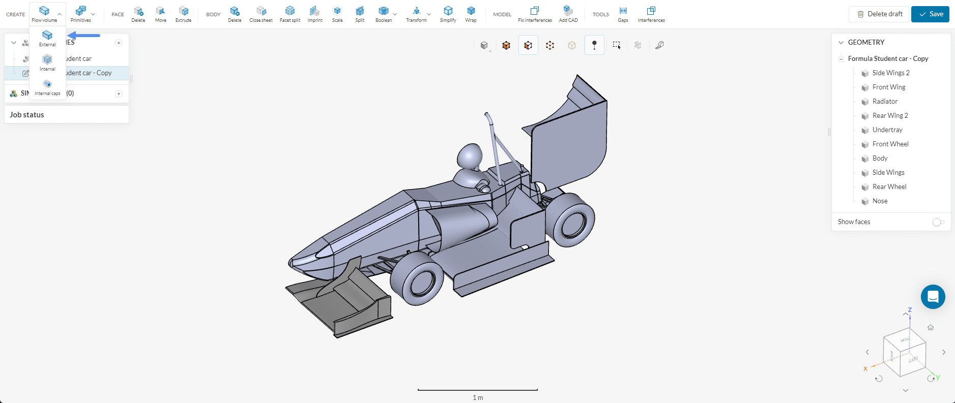
Create an External flow volume extraction first.
The size of the domain is chosen according to the reference length (L) of the model. Here, the reference length is the horizontal distance from the tip of the nose, to the back of the rear wing. As a rule of thumb, the following values can be used:
- Downstream: 8-10 times the length of the vehicle;
- Upstream: 3-5 times the length of the vehicle;
- As much as necessary in the negative z-direction, so that the ground can be tangent to the wheels;
- Other directions: 3 times the length of the vehicle.
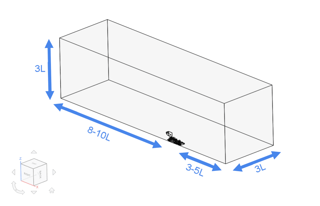
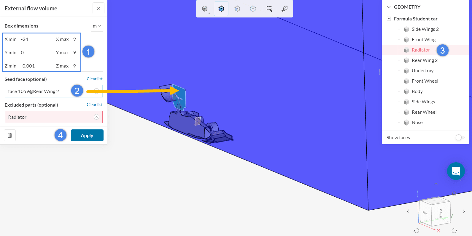
- Enter the following dimensions that appear in the figure below, according to the recommended sizing that was introduced before;
- Select one of the spoiler faces as a Seed face;
- Enable the Excluded parts assignment, assigning it to the ‘Radiator’ volume;
- Create the domain by clicking ‘Apply’.
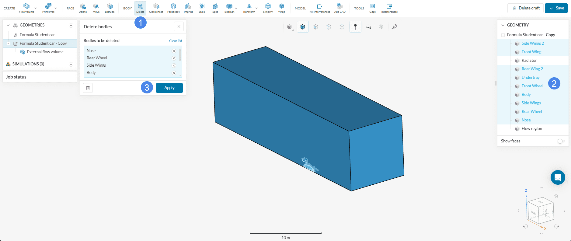
We will use the Delete body feature afterward, to make sure only the flow region and the cell zone remain in the final version.
As a result, only the Radiator and the Flow region will be left in the model. Press ‘Save’ to save the copy as a new version of the CAD model.
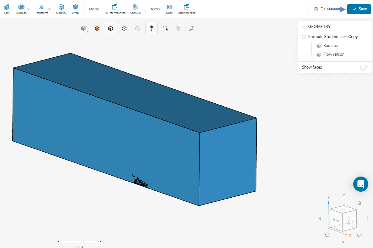
The final version will appear as ‘Copy of Formula Student car’. Before the setup, feel free to rename the new geometry as ‘Formula Student car’, and delete the one that is no longer necessary.
Did you know?
It is possible to rename a CAD model by clicking on it’s name and adding the name title:
Also, a geometry can be deleted by clicking on the trash icon, as you can see below:
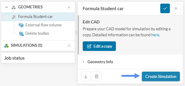
1.1 Create the Simulation
To get started, click on ‘Create a Simulation’:
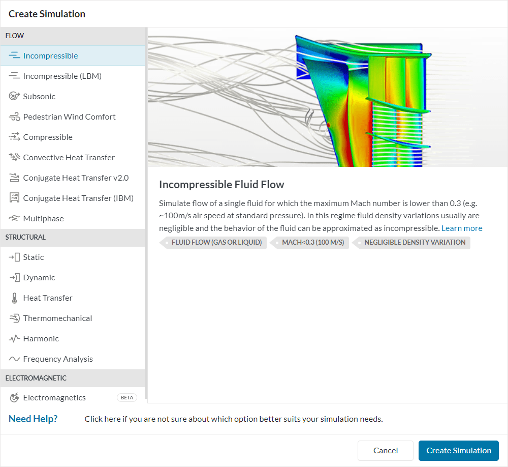
Doing so, the analysis type choice widget opens. Choose ‘Incompressible’ as the analysis type. It can be used for cases where the Mach number remains lower than 0.3 in the entire domain, which will be the case for this tutorial. Proceed by clicking on the ‘Create Simulation’ button:
The simulation tree will be visible on the left-hand side panel. We have to set up all entries, to be able to run the simulation. In this tutorial, we want to calculate the steady-state solution, which is independent of time. SimScale also supports transient analysis, which allows the calculation of time-dependent results.
The global settings of the simulation remain as default:
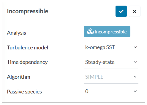
Did you know?
The k-omega SST turbulence model is recommended for external aerodynamics cases.
It works as a blend between the k-omega and k-epsilon models. The k-omega model is predominant in the near-wall, switching to the k-epsilon model in the free-stream.
Find more information about the k-omega SST model in this documentation page.
1.2 Create Saved Selections
Saved selections are groups of faces or volumes. They’re particularly helpful when the same group of faces is used several times during the simulation setup. The user can quickly select a given group of entities at once whenever they need to be assigned to a condition.
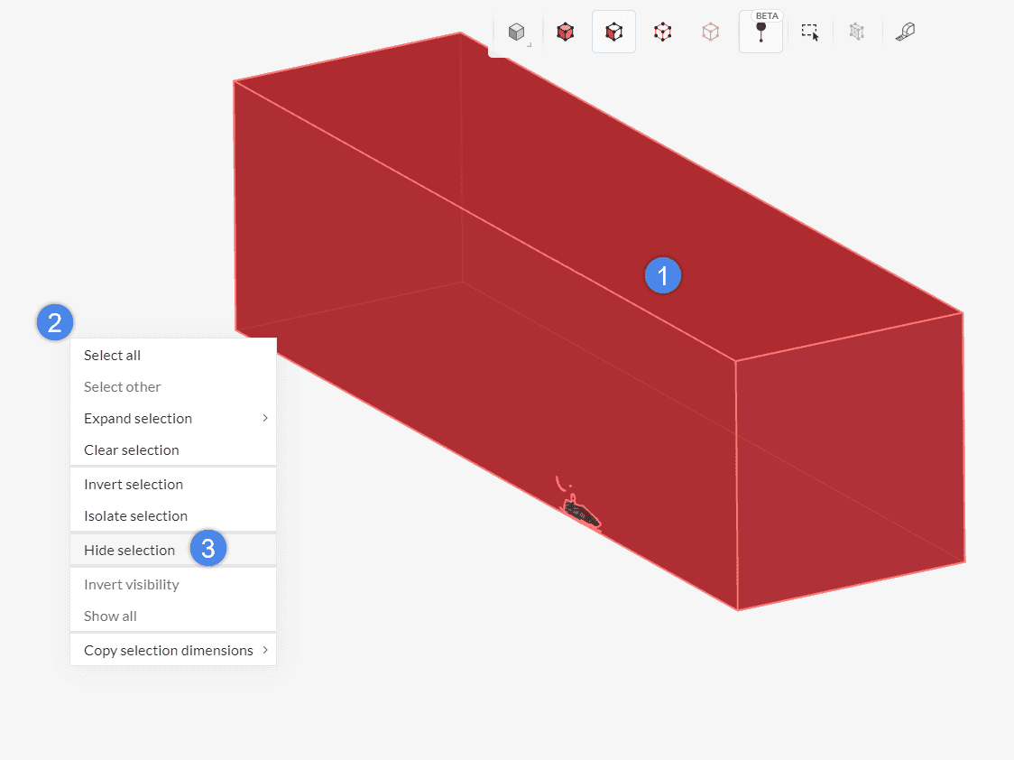
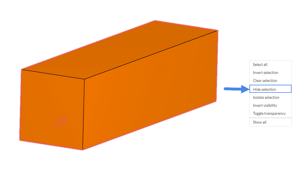
For this tutorial, three saved selections will be used, one including all the faces of the Formula Student car, and one for each wheel. First, hide the walls of the domain by selecting all of them (the face color must turn red), then right-clicking in the Workbench, and choosing the ‘Hide selection‘ option:
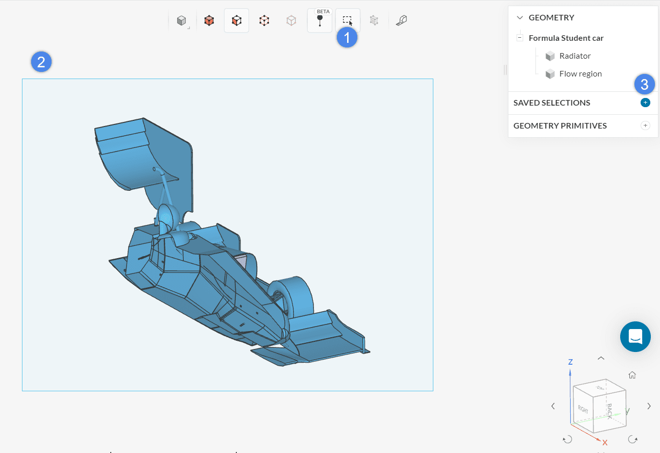
Activate the box selection and drag the cursor across the screen until all the remaining faces turn red. Then click on the ‘+’ icon next to Saved selections. Name it as ‘Full car’.
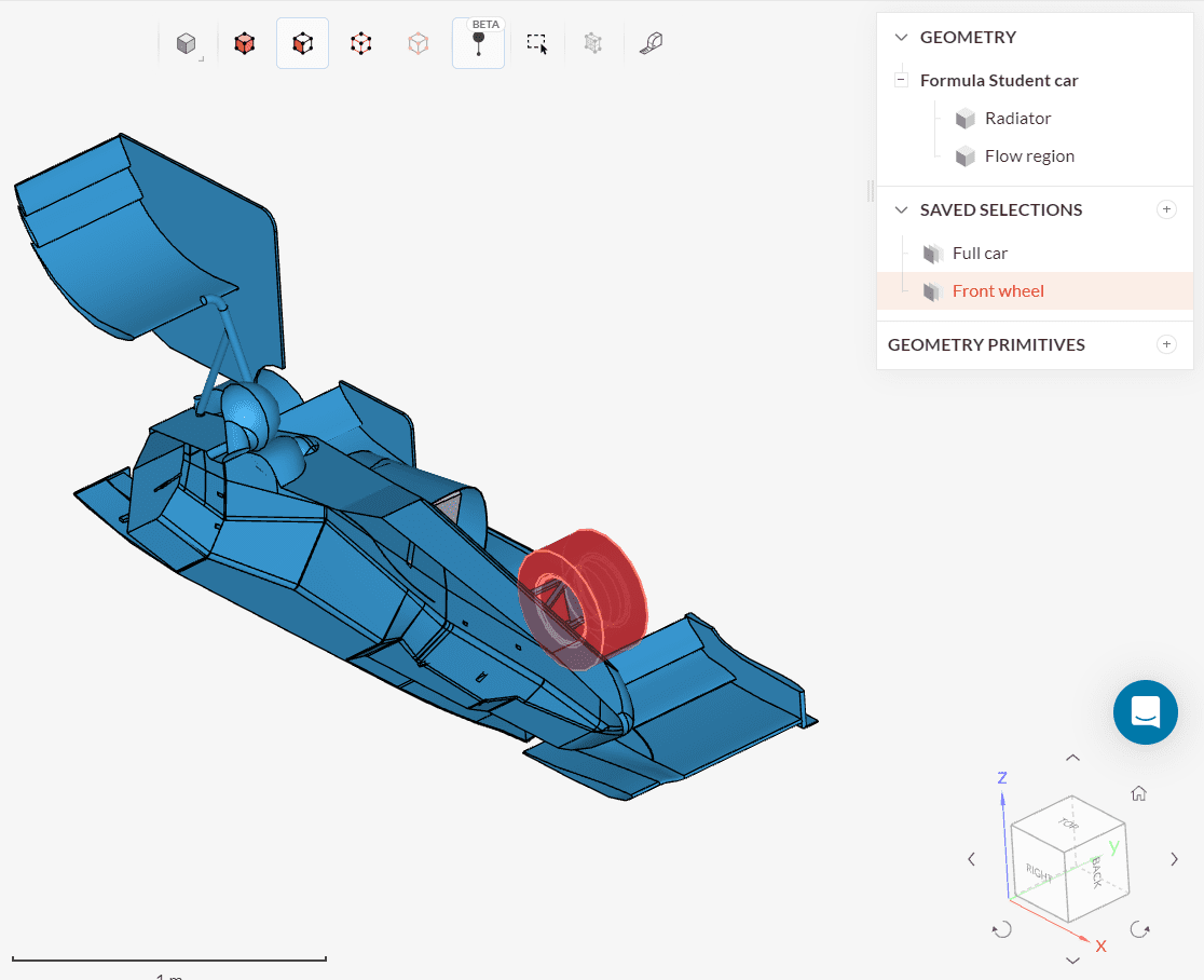
Proceed to create a set for the front and rear wheels too. Each wheel consists of 11 faces, and we will need to rotate and adjust the model in order to click on all of them before the set creation. The following photo shows how the saved selection of the front wheel should appear afterward, when everything else is hidden. See how the faces on the inside were included too:
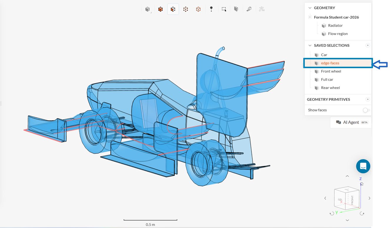
After creating the selection for the Front and rear wheels , now create the last selection for the small and thin surfaces of the spoiler trailing edges and others in the model.
See the below image to identify which ones are selected. In total there will be about 17 surfaces , that include 9 of the spoiler trailing edges and rest as shown.
These will be important during the meshing step for additional refinements.
2. Assigning the Material and Boundary Conditions
Now we are ready to set up the physics of the simulation.
2.1 Define a Material
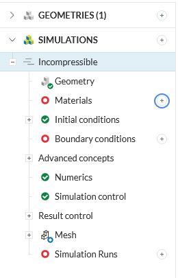
In the simulation tree, click on the ‘+’ icon next to Materials:
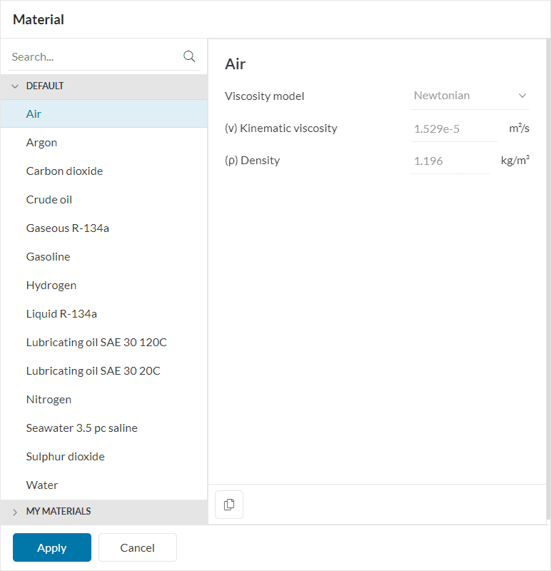
Choose ‘Air‘ in the panel that pops up and click ‘Apply’:
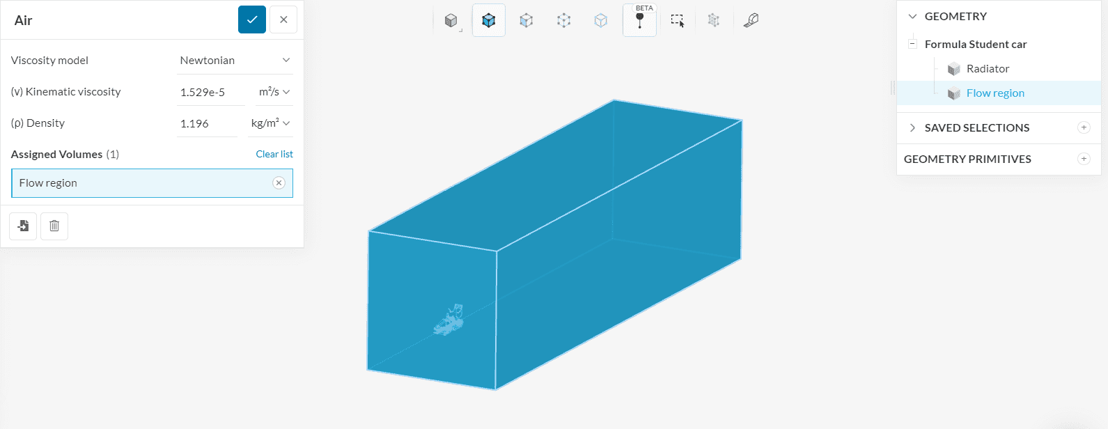
To assign the flow region as air, click on ‘Flow region’ under the scene tree as shown below. Leave the properties as default:
2.2 Assign the Boundary Conditions
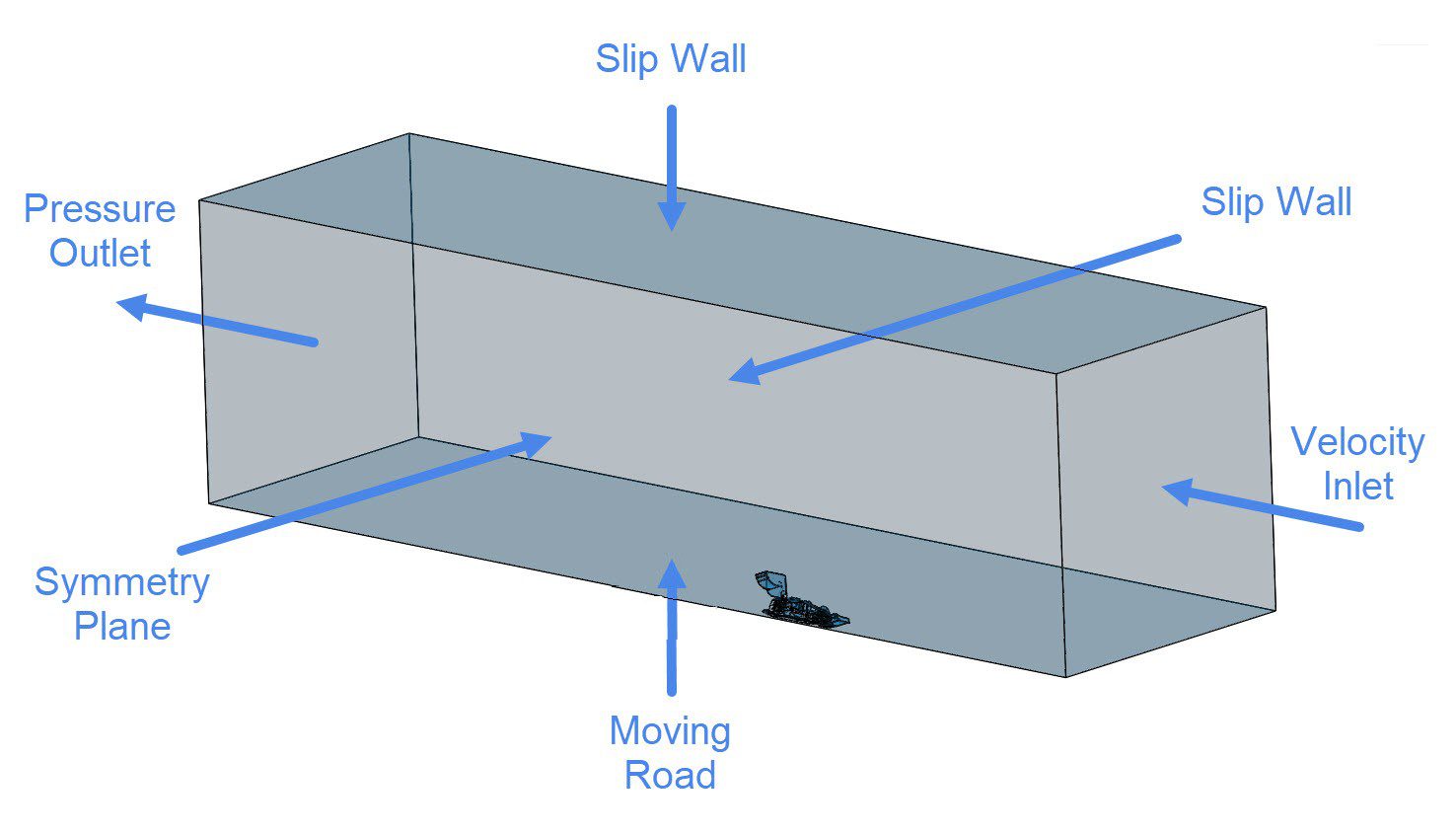
The physical situation simulated is a straight line movement with 15 (m over s). An overview of the boundary conditions for the domain can be seen below:
Similarly, for the car walls, the following boundary conditions are applied:
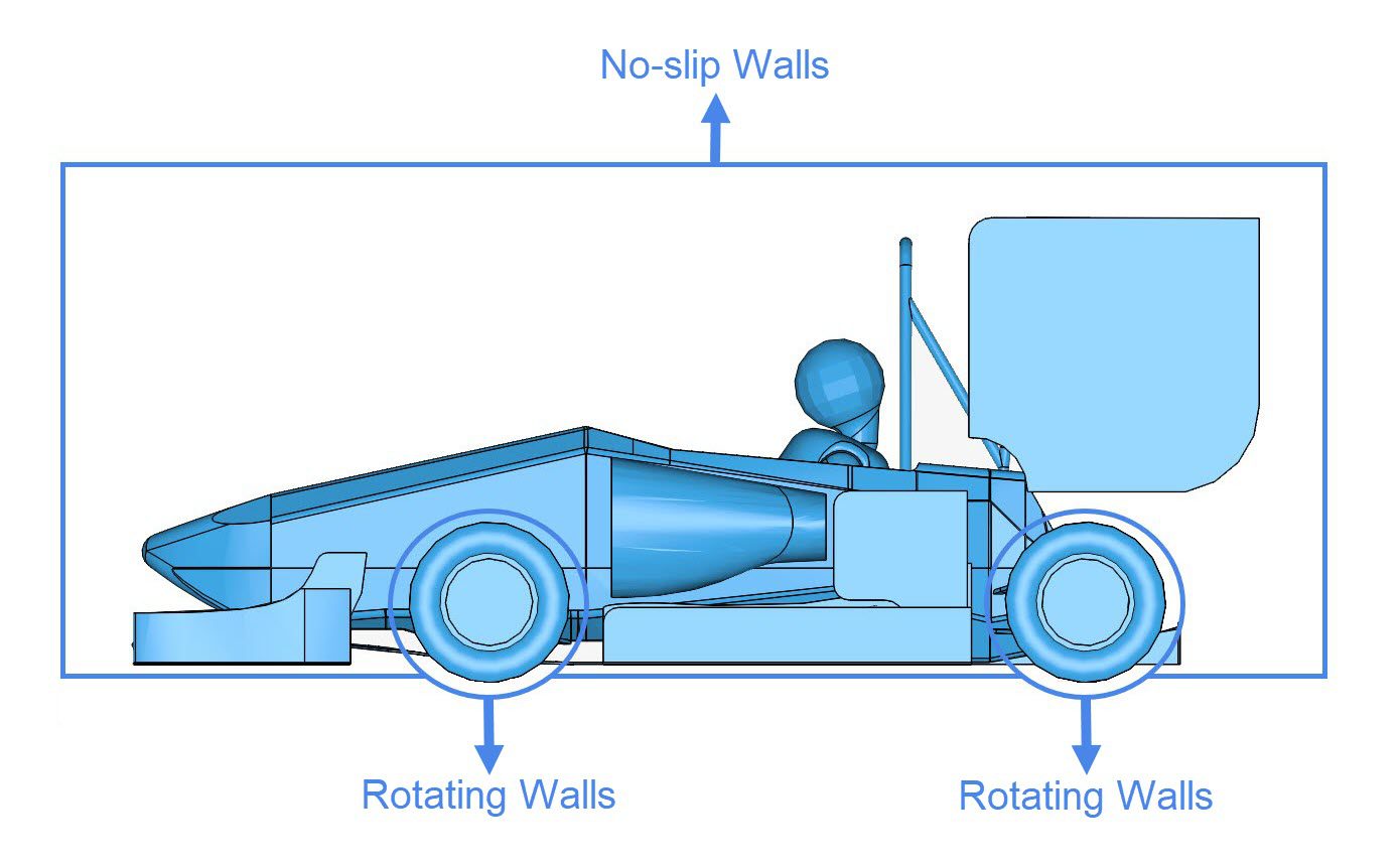
Except for the wheels, all other faces of the car will receive a no-slip wall boundary condition.
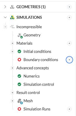
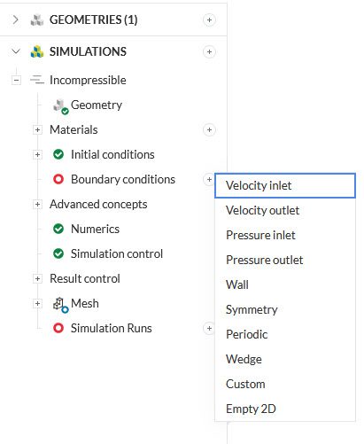
To create a boundary condition, click on the ‘+’ icon next to Boundary conditions, and select the desired type from the drop-down menu.
a. Velocity Inlet
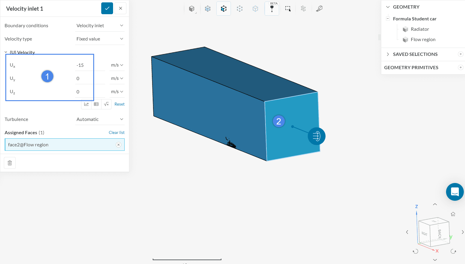
The straight-line simulation of a breeze-less environment can be achieved by setting a velocity inlet boundary condition at the frontal face of the domain. First, add a ‘Velocity inlet’ boundary condition from the menu:
The velocity value is 15 (m over s), and it represents the speed of the vehicle. It must be set according to the orientation cube, that is placed at the bottom right of the Workbench. Here, the air travels towards the negative x-direction, so (U_x) should be set to -15 (m over s), and the remaining components are set to 0 (m over s):
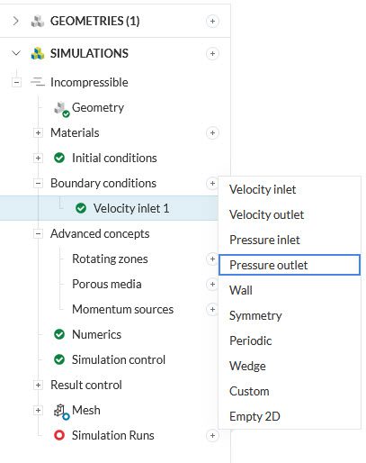
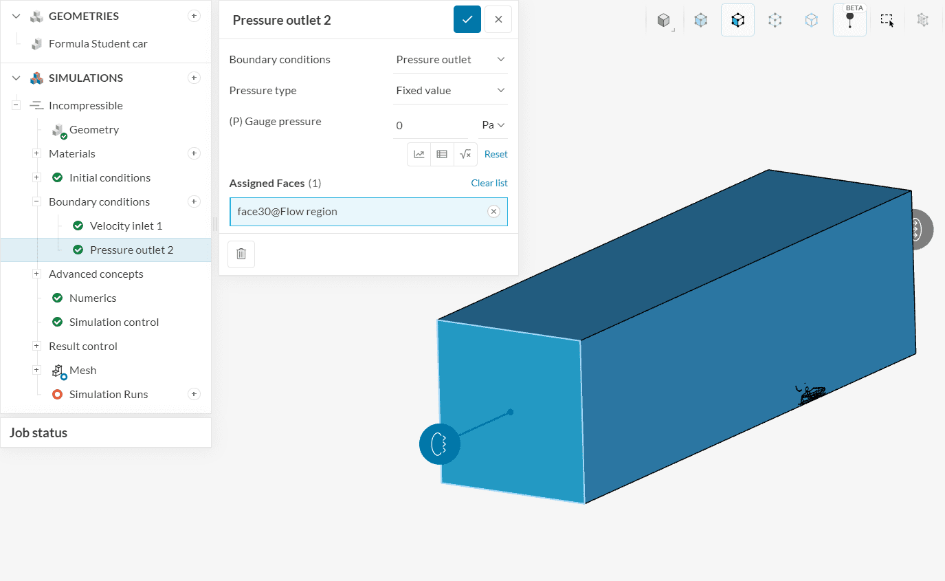
b. Pressure Outlet
As seen in the rest of the incompressible fluid dynamics tutorials, the most common boundary condition for the outlet of an external aerodynamics case is a zero Dirichlet condition for the gauge pressure. Proceed by selecting the ‘Pressure outlet‘ on the menu.
Rotate the CAD model and assign the condition on the outlet:
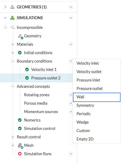
c. Walls: Slip Condition
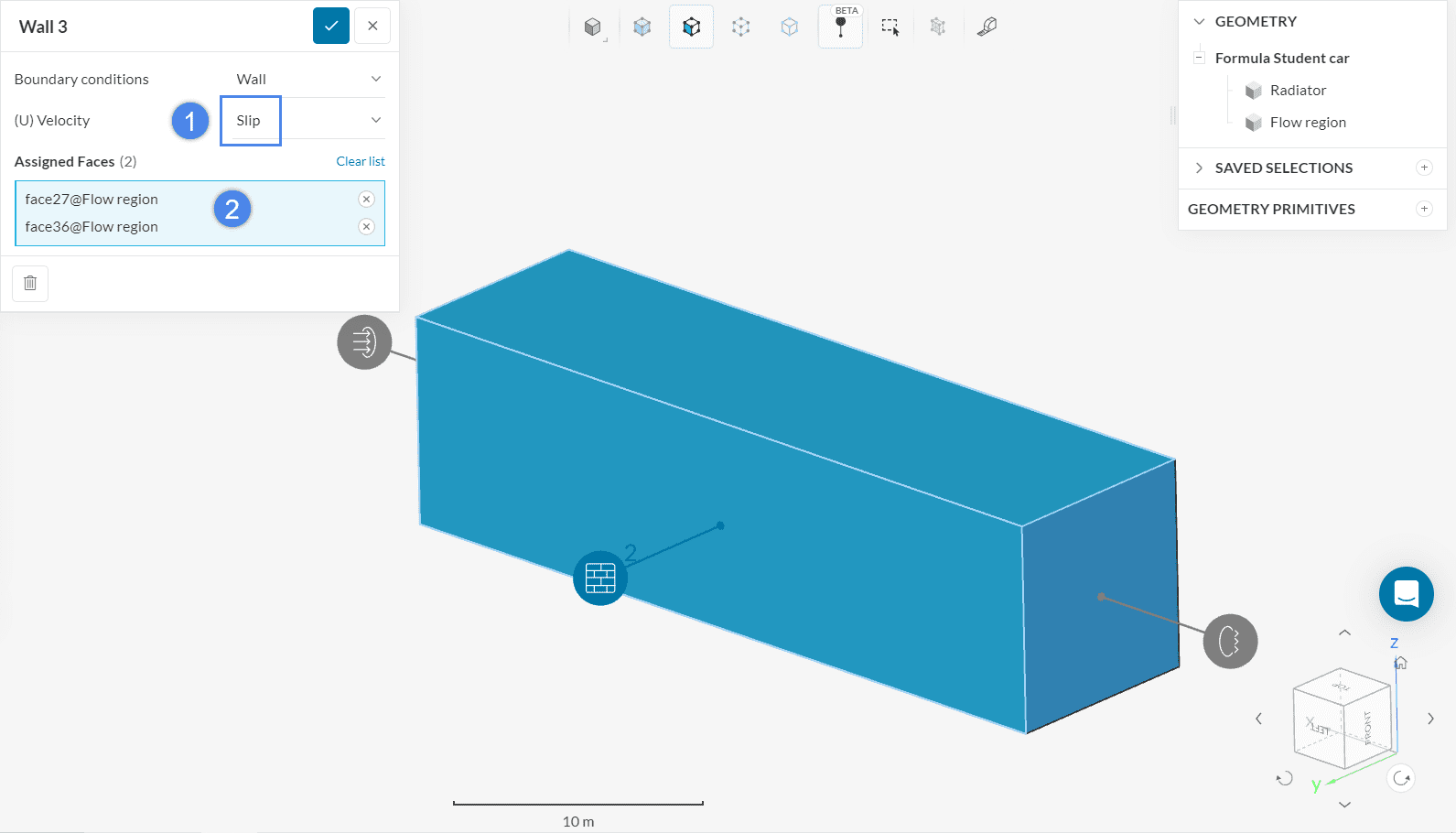
There are many types of wall conditions to use and all of them can be checked here. The top and right faces of the domain represent the open-air environment, and by setting the wall velocity to ‘Slip‘, its normal component is erased, and the tangential components remain untouched. Select the ‘Wall‘ category from the menu first:
Change the type of the wall by setting the (U) Velocity option, to ‘Slip‘.
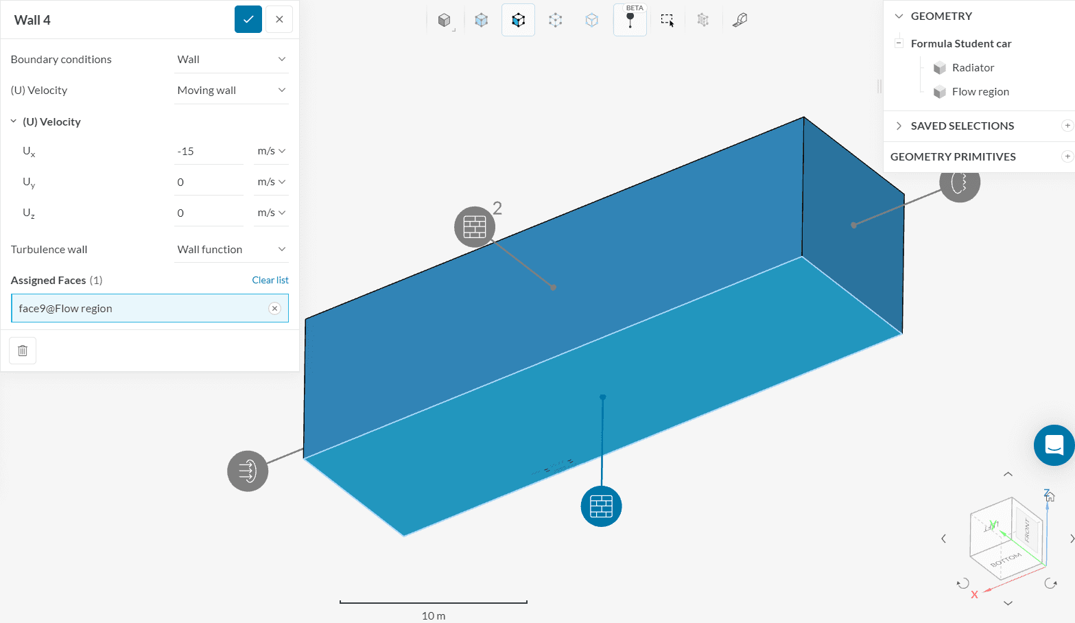
d. Wall: Moving Wall
Another use of the wall category is to model a moving surface, like the ground.
- For this set, switch the (U) Velocity to ‘Moving wall‘;
- The components of the velocity are treated exactly like the flow inlet.
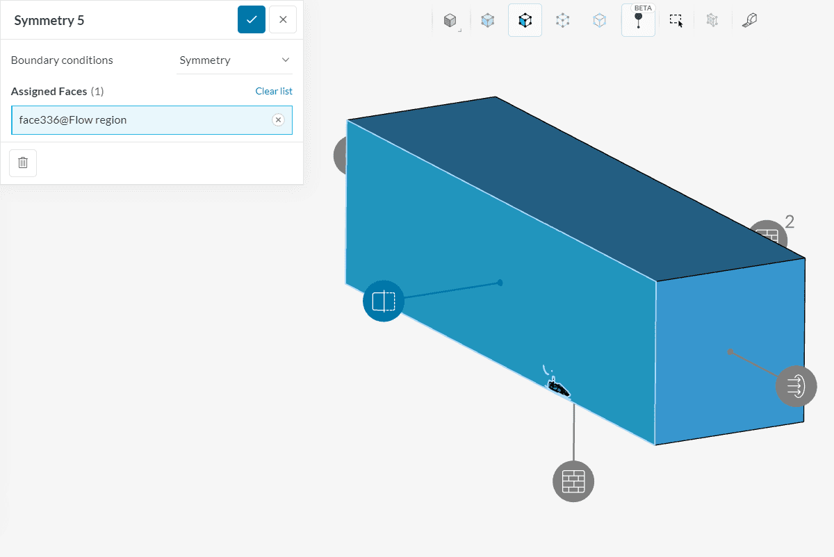
e. Symmetry
We are using half the Formula Student car model to save resources. Set the plane that is coincident with the cut surface as symmetry to indicate that the domain is mirrored. Select ‘Symmetry‘ from the Boundary conditions menu:
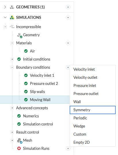
Then click on the respective side of the domain to set it as the mirroring plane:
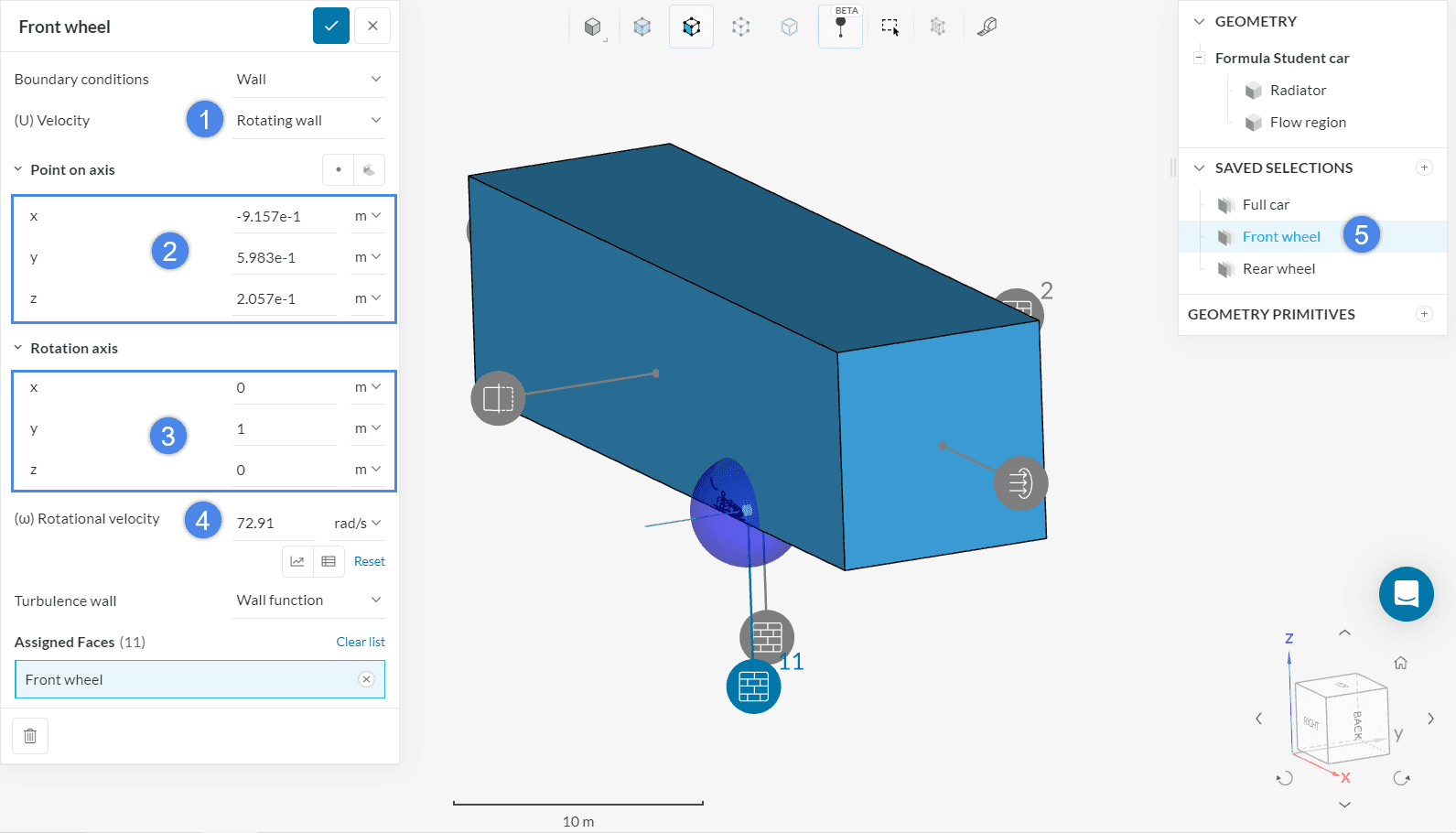
f. Wall: Rotating Wall – Front Wheel
For each one of the two wheels, we will create a new wall set, but this time, it will be modeled as a rotating wall.
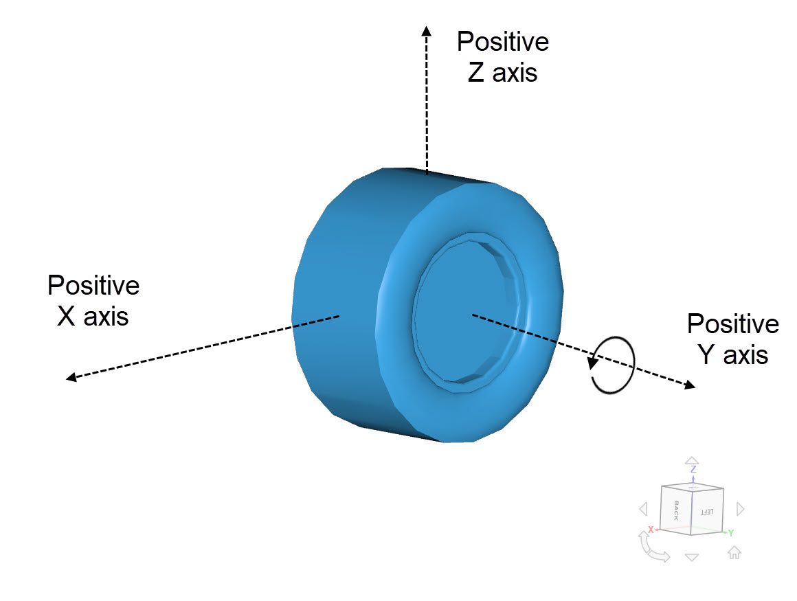
For the setting of the rotation axis, we will be using the right-hand rule. Use the following figure as reference:
- Change the (U) Velocity to ‘Rotating wall‘;
- Set the coordinates of the wheel’s center of rotation. This can be measured in a CAD software. For this case, enter the following values:
- (x): -0.91567 (m)
- (y): 0.5983 (m)
- (z): 0.20574 (m)
- Once again, the orientation cube indicates the correct direction of the rotation. Here, the car travels parallel to the positive (x) direction, so according to the right-hand rule, the rotation axis is the (y ) direction;
- The rotational velocity is calculated with the formula: (ω) = (U over r ), where:
- (U): the linear velocity
- (r): the radius of the wheel
- Select the ‘Front wheel‘ saved selection from the geometry tree.
g. Wall: Rotating Wall – Rear Wheel
The same procedure as before is followed for the rear wheel set. This time, the center of rotation coordinates are:
- (x): -2.44567 (m)
- (y): 0.5583 (m)
- (z): 0.20574 (m)
Select the ‘Rear wheel’ saved selection at the end:

2.3. Advanced Concepts
Note
If you are using your own model, that does not include a radiator, you can skip this section.
A radiator can be modeled as a porous media. There are different types, and each approach is described in this knowledge base article.
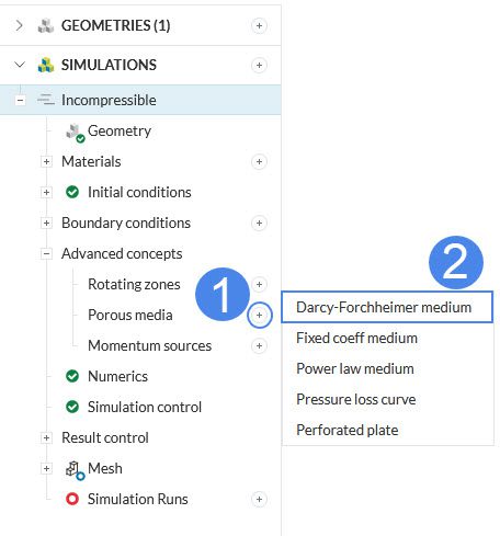
We will set four sections of settings for the porous medium, based on the Radiator’s placement and experimental data. The advanced concept can be either assigned to a volume, as in this project, or to user-created geometry primitive, like a cartesian box.
Have a look at this guide to learn more on how to set up unit vectors for the porous media.
- The first section, (d), that stands for Darcy, is a linear resistance coefficient which has three entries, one for each direction. Apply the following values:
- (d_x): 98008228.5 ( 1 over m^2 )
- (d_y): 980082284.8 (1 over m^2 )
- (d_z): 980082284.8 (1 over m^2)
- The second section, (f), includes three more entries, the Forchheimer resistance coefficients.
- (f_x): 1050.8 ( 1 over m )
- (f_y): 10508.4 (1 over m )
- (f_z): 10508.4 (1 over m )
- For a radiator that is angled, the Orientation should be set to ‘Custom‘;
- The appropriate coordinates of the Unit vector x are:
- (x): -0.93256 (m)
- (y): 0.09751 (m)
- (z): 0.3476 (m)
- And for the Unit vector y:
- (x): 0.33942 (m)
- (y): 0.09119 (m)
- (z): 0.9362 (m)
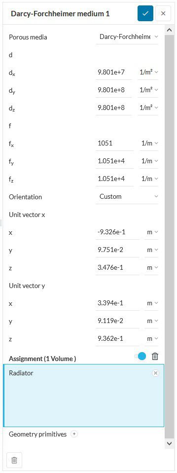
After the setup is complete, click on the ‘Radiator’ in the scene tree to assign the concept to it.
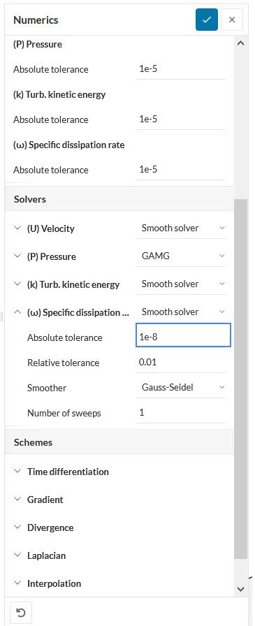
2.4. Set the Numerics & Simulation Control
The Numerics settings can be left as default, except from the absolute tolerance of (omega), as it was observed to reach values smaller than 1e-6.
- Go to the Solvers section;
- Expand the (ω) Specific dissipation rate;
- Set the absolute tolerance to ‘1e-8’.
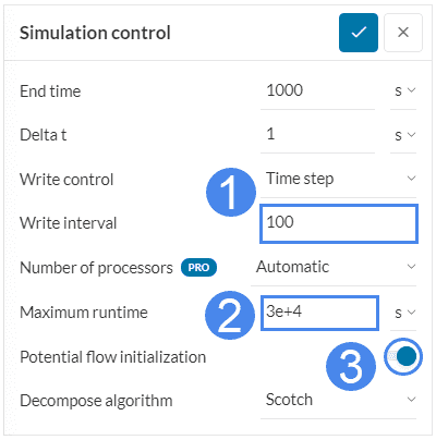
In the simulation tree, click on ‘Simulation control’ and configure it like this:
- In order to create an animation with the simulation results, set the Write interval to 100, then the results will be written every 100 iterations, resulting in a simulation with 10 frames (without including the initial condition at 0 (sec);
- Change the Maximum runtime for the simulation to ‘30000’ (sec);
- Enable ‘Potential foam initialization‘. This setting initializes the velocity field and enhances stability in the early iterations.
Did you know?
In a steady-state simulation, the End time and Delta t parameters control the number of iterations to be performed. With the default settings, a simulation consists of a total of 1000 iterations, which is enough for most simulations to converge.
For more notes on the simulation control settings, please visit the following page: Simulation Control for Fluid Analysis.
2.5. Results Control
This section is important for the post-processing of the simulation run. There are many different features under the Result Control that we can use to evaluate the vehicle’s performance.
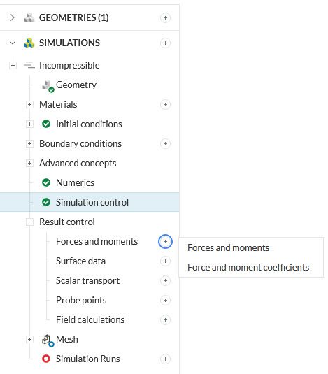
Forces and Moments
With the Forces and moments, we can extract the pressure, viscous and porous forces, and moments of various parts of the model.
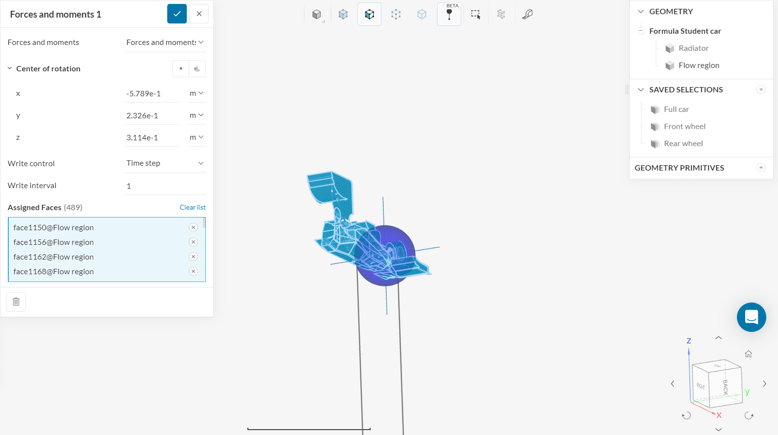
Lift and drag coefficients are some of the most important parameters when evaluating the performance of a vehicle. The center of rotation can be calculated externally using the CAD software, and for this specific geometry it has the following coordinates:
- (x): -0.57895 (m)
- (y): 0.23262 (m)
- (z): 0.31138 (m)
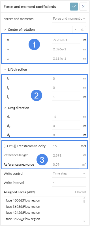
Force and Moment Coefficients
We can also create a Force and moment coefficients set, to monitor the drag and lift coefficients, (C_d) and (C_l) respectively.
- For this set, the coordinates of the center of rotation remain as in Table 1.
- The direction of lift, drag and pitch are set according to the coordinate cube:
- Set the positive z-axis as the Lift direction by assigning ‘1’. The other axis receive a value of ‘0’;
- Set the positive x-axis as the Drag direction by assigning ‘1’. The other axis receive a value of ‘0’;
- Set the positive y-axis as the Pitch direction by assigning ‘1’. The other axis receive a value of ‘0’;
- Apart from these, some new inputs must be also added, according to the boundary conditions and the characteristics of the Formula Student car:
- (|U<∞>|) Freestream velocity magnitude: 15 (m over s)
- Reference length: 2.891 (m), calculated with the CAD software
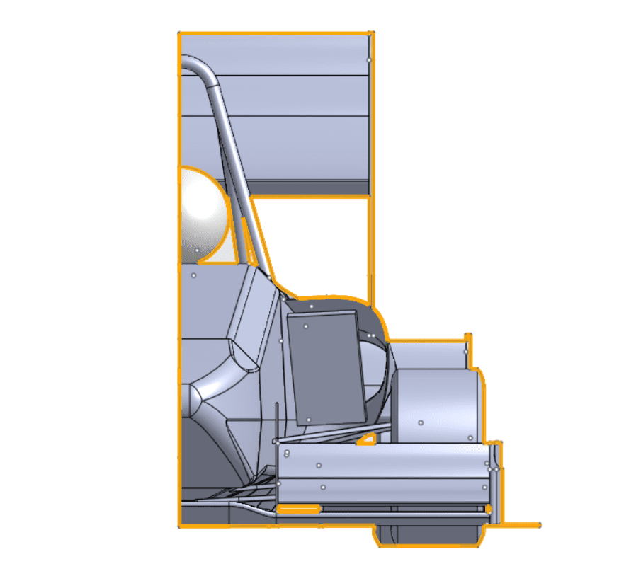
- Reference Area value: 0.59 (m^2)
The Reference area value is a projection of the frontal vehicle area onto a plane. When using half the Formula Student car geometry, the area projection must account only for half of the model. One way to do it is to create a sketch and project the faces on the plane. Then check the designed area.
The final Forces and moment coefficients panel should appear like this:
Assign the result control to all of the car faces except the Radiator, like we did for the previous Result control set.
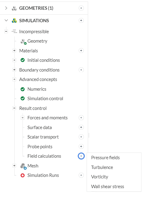
Field Calculations
Include more parameters in the results by clicking on the ‘+‘ icon and selecting each one of the entries. With the turbulence, for example, we will be able to check the (y^+) value and make sure it is below 1.
Important
Be careful when setting up the result control parameters, as they are used by the algorithm to calculate the drag and lift coefficients.
For the drag and lift formulas, and more examples on how to set up the forces and moment coefficients result control, please refer to the following articles:
How to analyze the pitch, lift, and drag coefficients?
Why are my lift and drag coefficients too big/small?
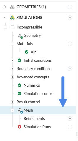
3. Mesh
When the simulation is created with the standard mesher, the mesh setup is placed right before the end, as the boundary conditions were previously set on the faces of the enclosure. This means that even if the mesh is changed and re-generated, we will not have to re-assign the boundary conditions. Click on ‘Mesh’.
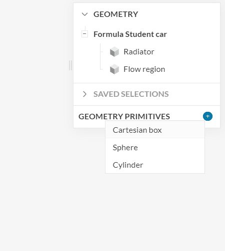
3.1. Create Geometry Primitives
Initially, we will create two cartesian boxes and region refinements will be assigned to each one of them later.
Click on the ‘+‘ button next to Geometry primitives, and choose the ‘Cartesian Box‘ option like below:
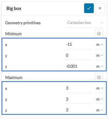
The first cartesian box is the biggest of the two and has the following dimensions, that are set in the same way as the background mesh box, which is by having a maximum and minimum value for each direction:
- Minimum x value: ‘-15’ (m)
- Minimum y value: ‘0’ (m)
- Minimum z value: ‘-0.001’ (m)
- Maximum x value: ‘3’ (m)
- Maximum y value: ‘3’ (m)
- Maximum z value: ‘3’ (m)
Then create the small box, with the following dimensions:
- Minimum x value: ‘-6’ (m)
- Minimum y value: ‘0’ (m)
- Minimum z value: ‘-0.001’ (m)
- Maximum x value: ‘1’ (m)
- Maximum y value: ‘1’ (m)
- Maximum z value: ‘1.5’ (m)

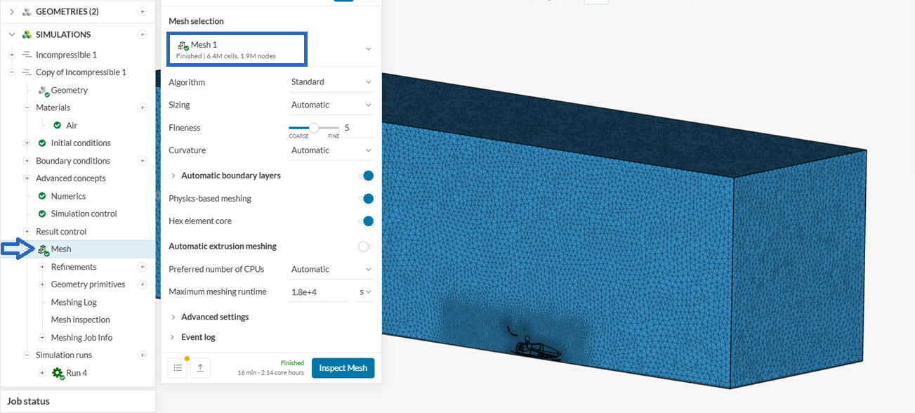
3.2. Apply the Main Mesh Settings
Go back to the Mesh panel, and make the following changes:
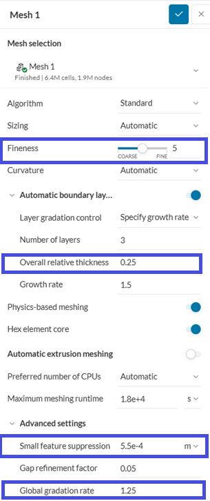
- Keep the mesh level of Fineness to ‘5’ for a moderate initial mesh.
- Expand the ‘Automatic boundary layers’ section to prepare the boundary layer mesh creation. For this case, use the default method with 3 layers for the default wall function approach mesh.
- Adjust the overall thickness to 0.25
- Keep the ‘Physics-based meshing’ setting and the ‘Hex element core’ setting toggled ON.
- Expand the ‘Advanced settings’ section to control the meshing. Set the Small feature suppression to ‘0.00055’ (m). This will be the smallest edge resolved, which means that the fineness of the mesh will be reduced, reserving computational resources.
- Change Global gradation rate to 1.25
Resolving the boundary layer
If you are using your own model, you can use this page to manually calculate the first layer thickness according to your case.
3.3. Add Refinements
For the standard mesher, several refinement options can be selected by the user to get the required mesh. These are all specified under the Refinements mesh sub-tree.
Volume Custom Sizing
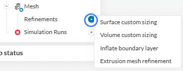
The volume custom sizing is used to refine the volume mesh for one or more user-specified volume regions under Geometry primitives. Add a Volume custom sizing by clicking on the ‘+’ icon next to Refinements, and then choosing the ‘Volume custom sizing’ option.
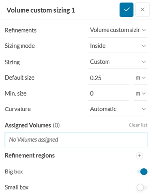
The first volume custom sizing that we will create is matched to the big cartesian box. The Sizing mode will be automatically set to Inside. This refines all volume mesh cells inside the surface up to specified default size. The surface needs to be closed for this to be possible.
- Set the Default size to ‘0.25′;
- Toggle on the ‘Big box‘ for the assignment.
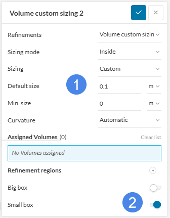
Then add a second volume custom sizing for the small cartesian box. This time:
- Set the Default size to ‘0.1’;
- Toggle on the ‘Small box’ for the assignment.
Surface Custom Sizing
Add this type of surface refinement by clicking on the ‘+’ icon next to the Refinements, and then choosing the ‘Surface Custom Sizing’ option.
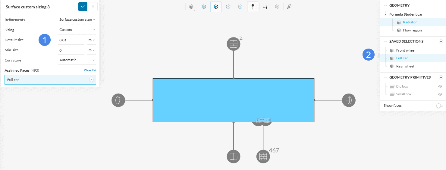
We will set a default size for the cells on the assigned surfaces.
- Set the Default size to ‘0.01’ (m);
- Assign the refinement to the whole vehicle by clicking on the ‘Full car’ saved selection as shown below.
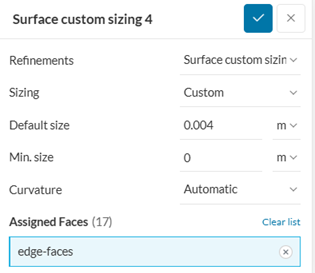
Then add a second surface custom sizing for the small surfaces. This time:
- Set the Sizing to Custom value of ‘0.004’ m;
- From the saved selections click the ‘edge-faces’ for the assignment
3.4. Generate Mesh
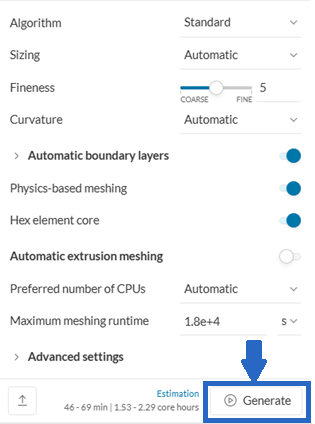
Go back to the main mesh tab. An estimation of the duration of the meshing procedure, the core hours that will be spent, as well as the size of the mesh, will appear. Click on the ‘Generate’ button to get started.
3.5. Meshing Results
After approximately 20 minutes, the mesh is ready, and the icon next to the Mesh section on the simulation tree will have a green checkmark. The Mesh total cell count should be around 6-7 million cells.
It is possible to zoom in to check the generated boundary layer or even create a mesh clip to inspect the interior of the mesh.

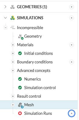
4. Start the Simulation
The simulation setup is now ready. We can proceed to create a new simulation run. To do so, click on the ‘+’ icon next to Simulation Runs.
This way, the mesh will be generated, and, afterward, the simulation run will start automatically. While the simulation results are being calculated, we can already have a look at the intermediate results in the post-processor. They are being updated in real-time!
There is also a link to the finished project at the end of the tutorial.
Caution
Upon starting a new simulation run you may see a warning :
“Some mesh elements have quality metrics outside the recommended ranges. We encourage you to investigate the mesh quality with the suggestions provided in the documentation.”
This can be ignored and you can start the run
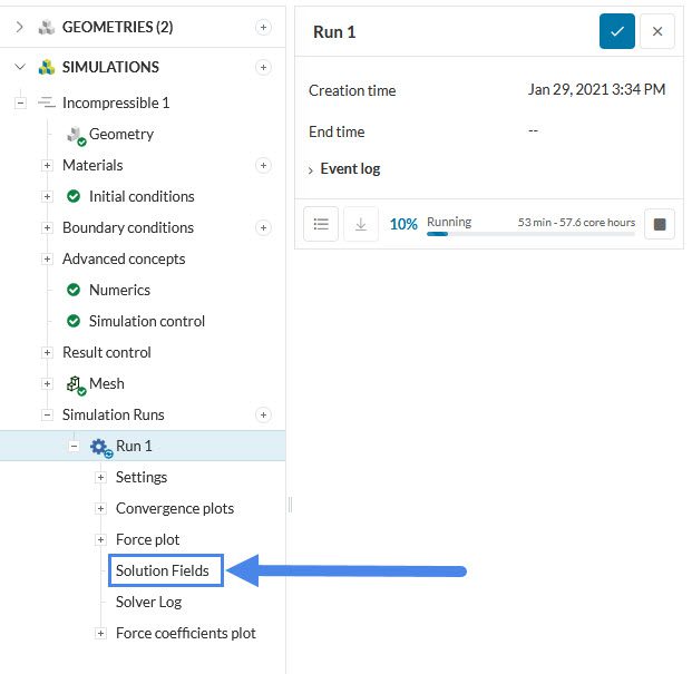
The simulation run takes an hour or so to finish, depending on the model that is used, and its complexity.
During the simulation, we can access the post-processing environment by clicking on ‘Solution Fields’ after expanding ‘Run 1‘:
5. Post-Processing
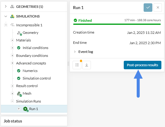
After the simulation is finished, we can extend Run 1 to check the results.
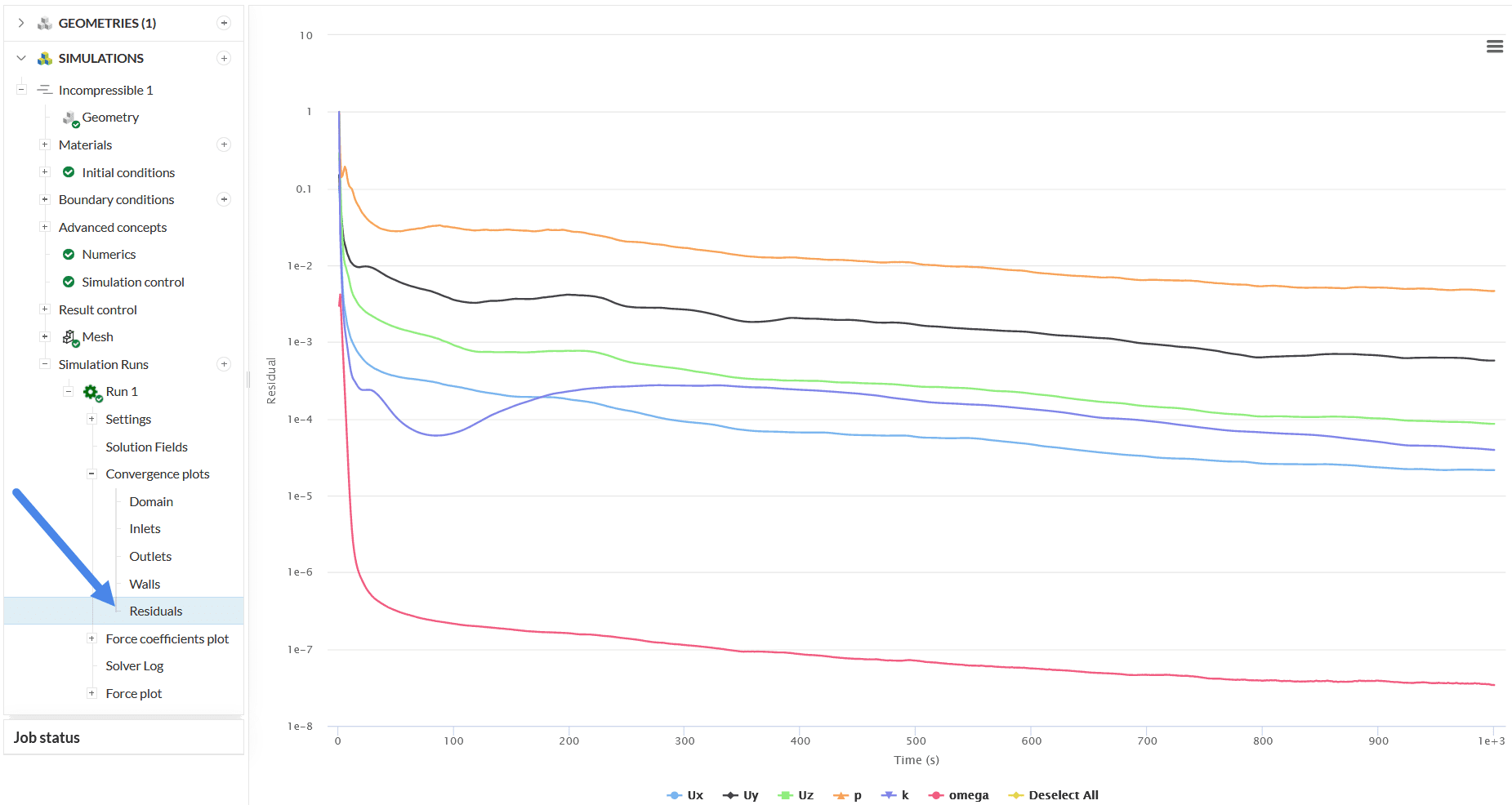
5.1. Convergence Plot
Make sure to check whether the simulation converged or not, by expanding the Convergence plots section, and then clicking on ‘Residuals‘.
5.2 Forces and Moments
The drag and lift are available in the ‘Forces and moments’ graph that appears after expanding Force plot:
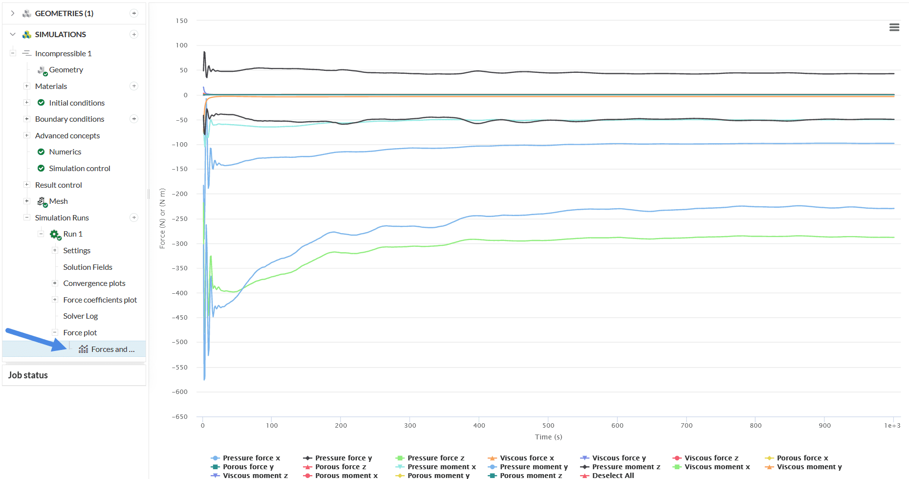
The plot shows us how the values are changing throughout the simulation process, as the iterations go on. In a converged simulation, the coefficients will stabilize around a value. Therefore, in a steady-state simulation, the intermediate results are important to assess convergence. The final converged solution is the one that should be analyzed to obtain the flow parameters.
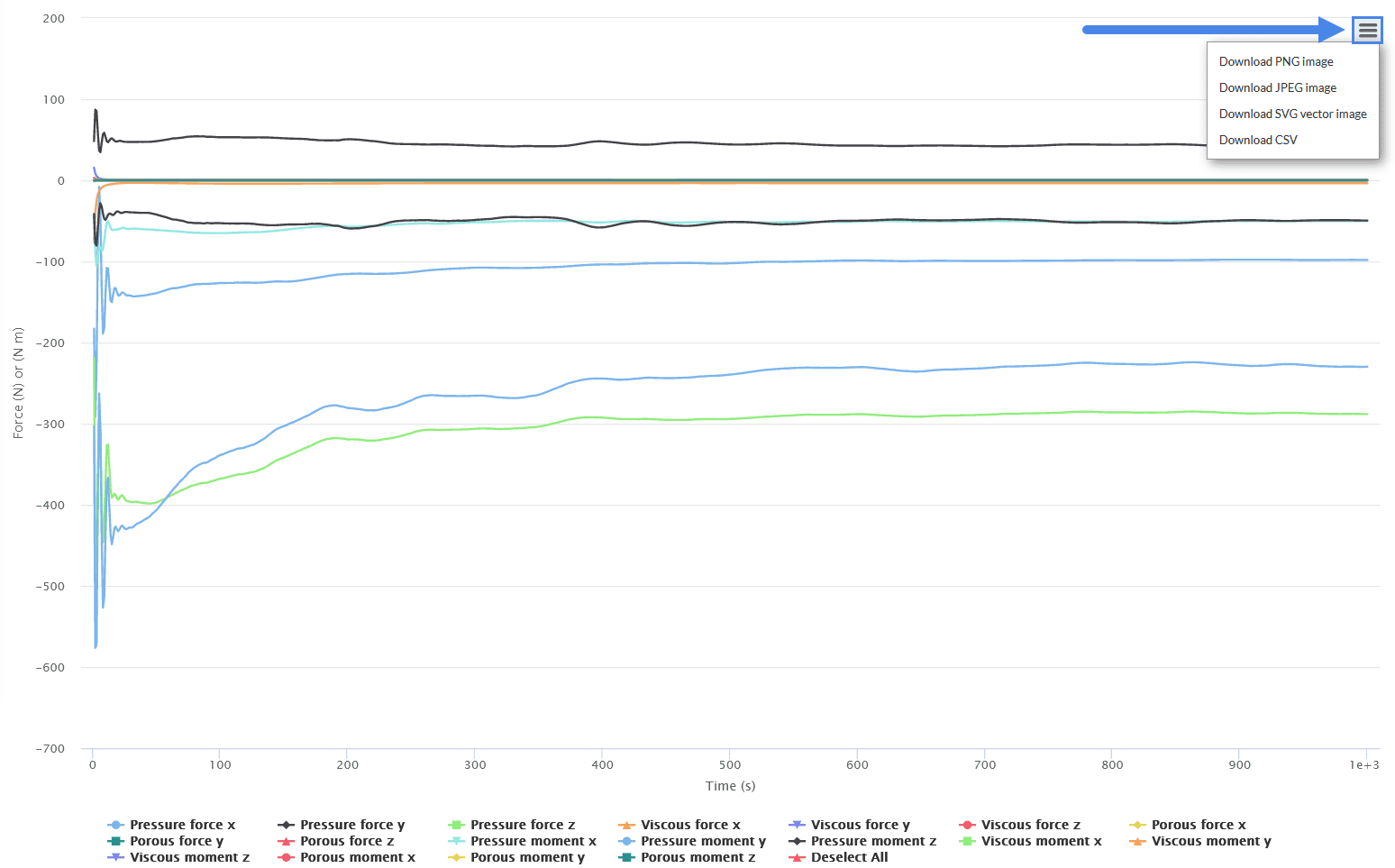
It is also possible to download the results in .csv format and analyze them with an external program, and get the average value from the final iterations. This can be done for all the plots by clicking on the icon at the top right of the plot, and selecting the format you want to export:
The same steps can be applied to the Force coefficients plots section too.
5.3 Post-Processing Interface
In order to enter the post-processor, click on the ‘Post-process results’ option:
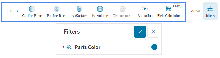
The first thing we might see is the whole domain, colored with pressure values. We can change the coloring, as shown in the next section, or use other features, in the Filters toolbar, and select one of the available choices.
Surface visualization (Parts Color)
Initially, click on the walls of the flow domain, right-click on the screen, and choose ‘Hide selection’, so only the Formula Student car is visible:
When the walls are hidden, we will see the pressure distribution on the car:
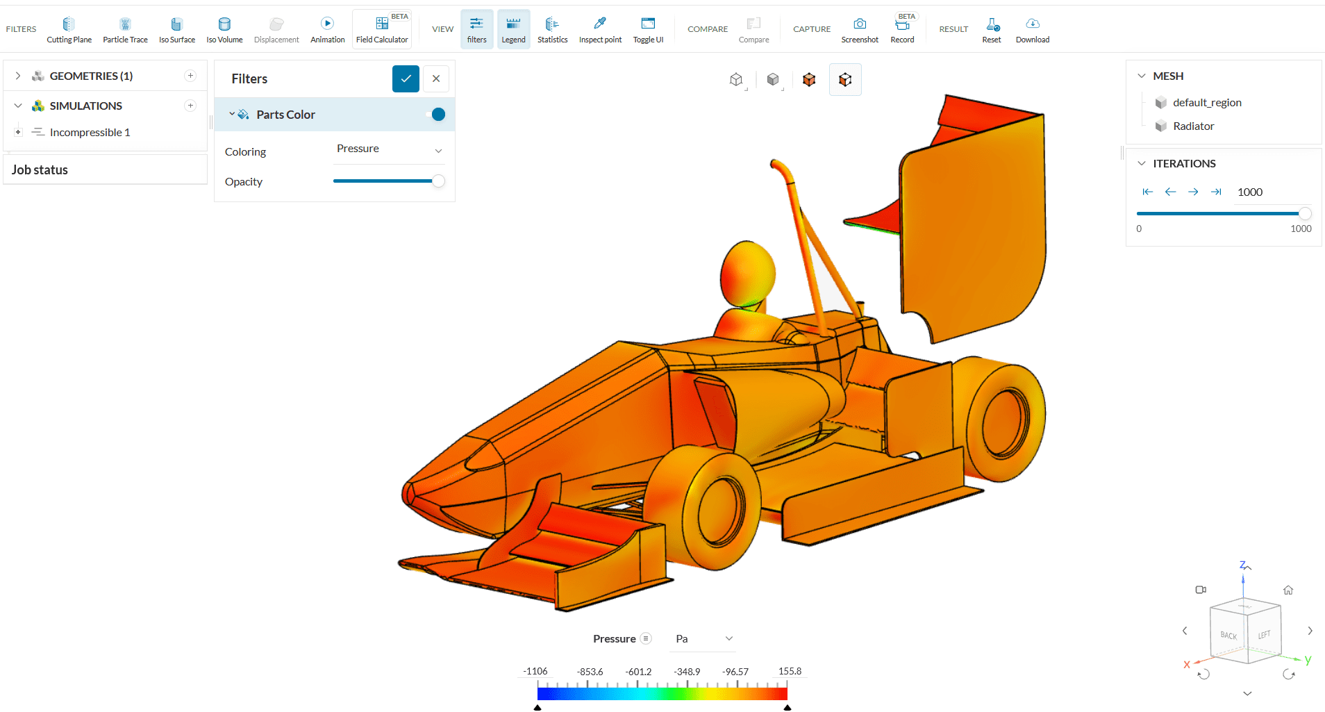
The warm-colored contours showcase the areas with the highest pressure values. As expected, these are the upper sides of the downforce-generating airfoils, as well as surfaces that are the first to come in contact with the freestream air, such as the nosecone, the driver’s body, etc.
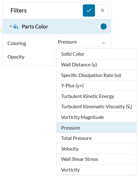
Pressure is not the only parameter that can be visualized on the model’s faces. We can switch to another parameter by changing the Coloring option.
Cutting Planes
We can check different slices of the flow region, by creating cutting planes. For example, we can visualize the velocity on a plane that cuts across the front wing.
- Position: Extend this section, so that the coordinates of the seed face can be selected.
- Orientation: We can either choose the axis that the plane will be normal to or extend the section to customize the direction;
- Coloring: By clicking on this, we can select the parameter we want to visualize. The following figure uses the magnitude of the velocity.
Hide the ‘Parts Color‘ and activate the ‘Clip model‘ option, so the only feature that appears is the slice we created:
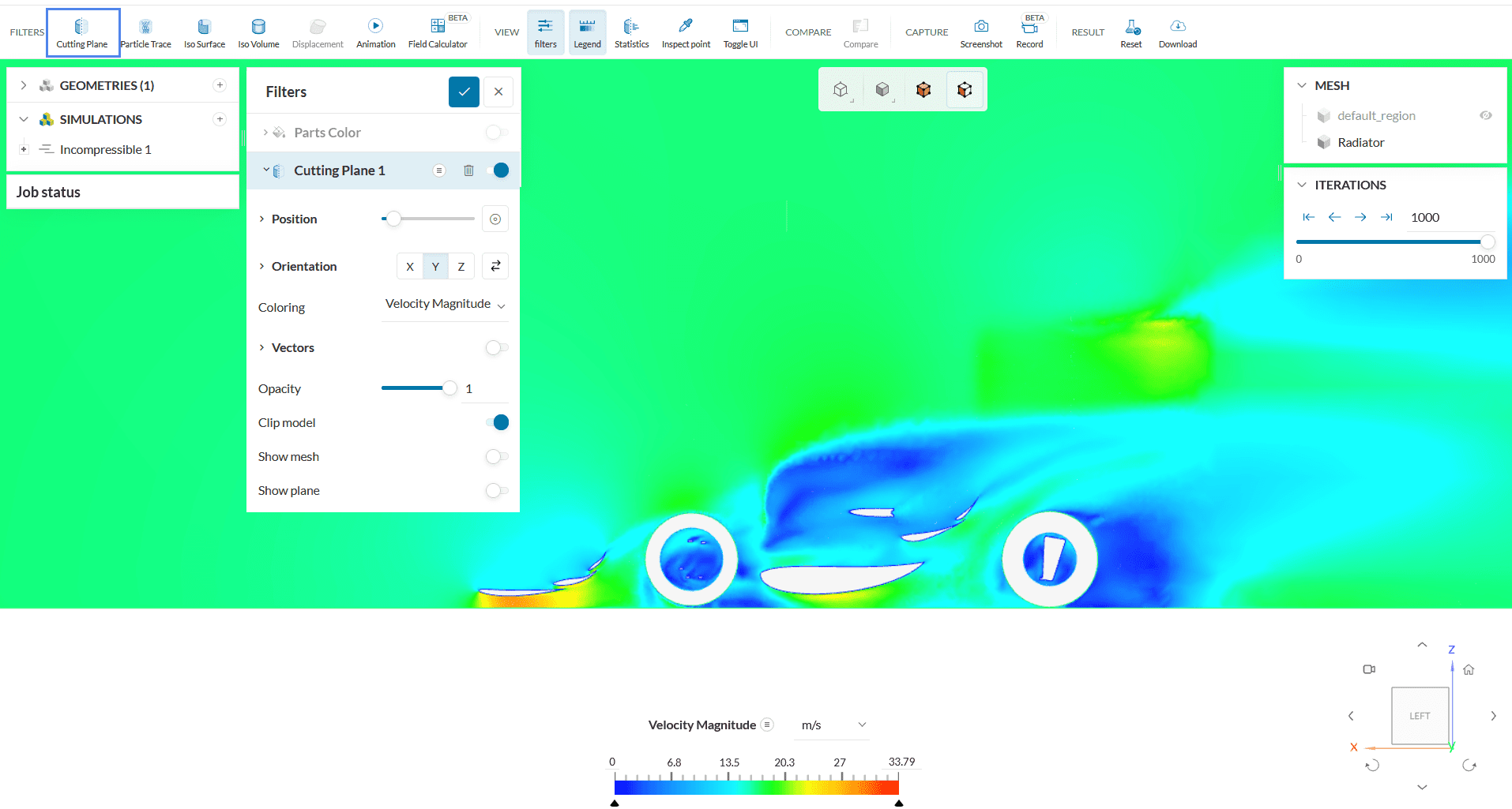
Suction regions with very low velocities can be analyzed with blue contours, as well as the acceleration of the flow below the front wing, which is a clear indication of downforce generation.
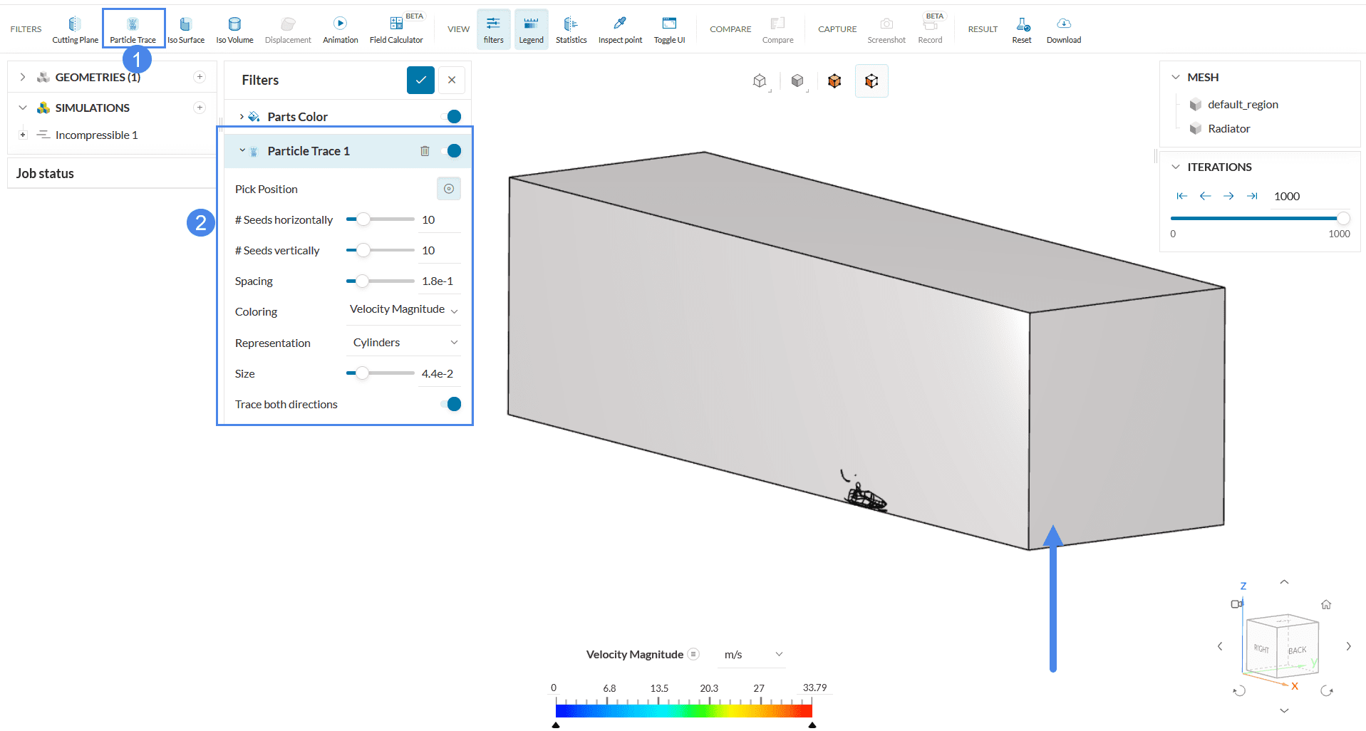
Particle Trace
One more useful feature is the streamlines. To create this, select ‘Particle Trace’ from the Filters toolbar. The whole domain will appear at first, and we will choose the position of the seed face, by clicking on the inlet, in front of the car. This will be the starting point of the streamlines:
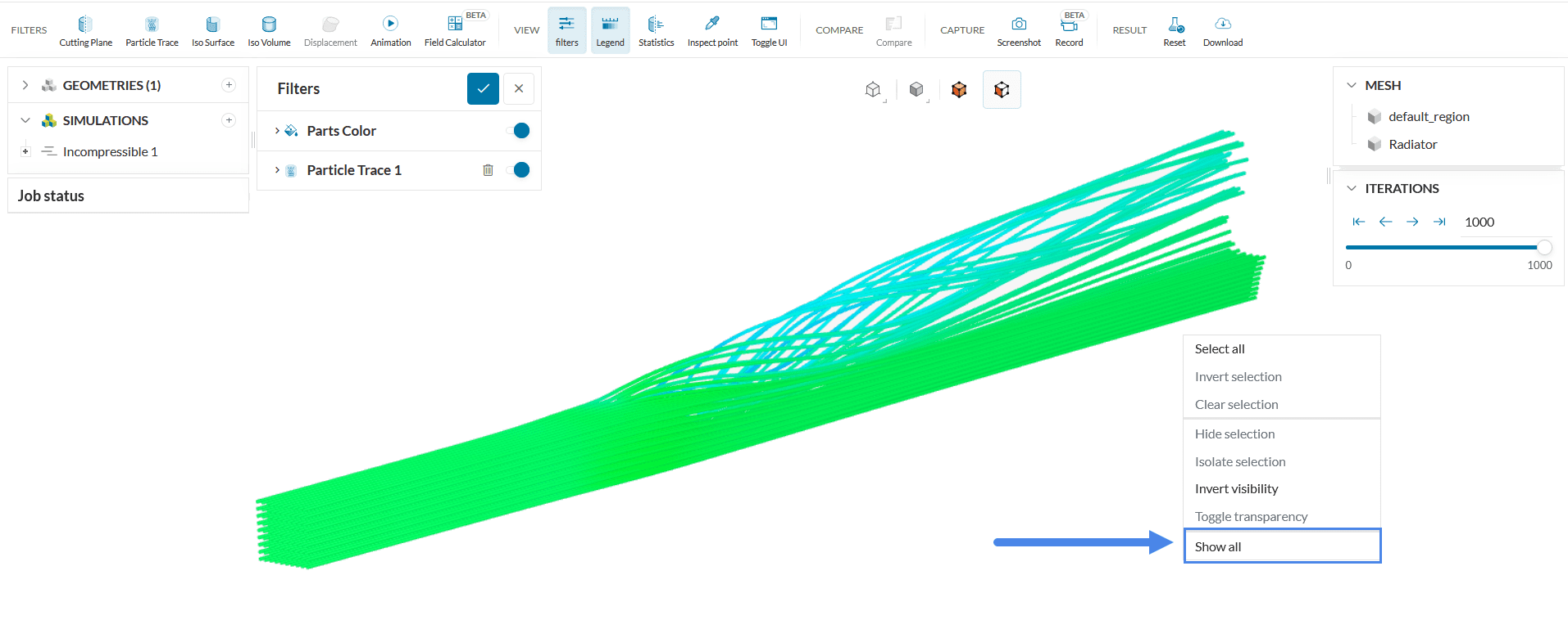
Only the streamlines and the radiator will be visible. Close the ‘Particle Trace 1’ tab, right-click on the workbench, and choose the ‘Show all’ option:
Proceed to select all six faces of the domain and hide them, like in Figure 65. Go back to the Particle Trace tab, and modify the number of particles under # Seeds horizontally and # Seeds vertically. For this tutorial, we can use ‘5’ points horizontally and ‘100’ points vertically. Change the Spacing of the streamlines to ‘5e-2’ and the size to ‘4e-3’.
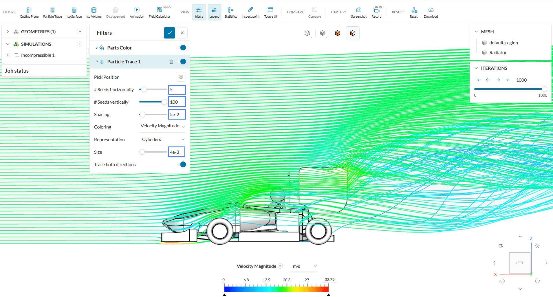
With streamlines, the flow around the complex structures can be better analyzed. Other than the velocity magnitude, the visualization of the vorticity on the streamlines can help with the recognition of the areas that need smarter design and optimization.
We can customize the streamlines and other features as we wish, by changing the inputs on each tab. Have a look at our post-processing guide to learn how to use it.
Congratulations! You finished the aerodynamic flow behavior of an FSAE car tutorial!
Note
If you have questions or suggestions, please reach out either via the forum or contact us directly.
Last updated: April 7th, 2026
Did this article solve your issue?
How can we do better?
We appreciate and value your feedback.


