The objective of this article is to explain how to predict Darcy and Forchheimer coefficients for perforated plates through curve-fitting, using experimental data.
Curve Fitting Approach
Pressure loss through the porous media is calculated by the following equation:
$$ \Delta P = \mu \cdot d \cdot L \cdot u + \frac{1 }{2} \cdot \rho \cdot f \cdot L \cdot u^{2} \tag{1}$$
where:
- \(\Delta P\) : Pressure drop \([Pa]\)
- \(\mu\) : Dynamic viscosity of fluid \([\frac{kg}{ms}]\)
- \(L\) : Thickness of perforated plate \([m]\)
- \(u\) : Velocity of fluid \([m/s]\)
- \(\rho\) : Density of fluid \([\frac{kg}{m^3}]\)
- \(d\) : Darcy coefficient
- \(f\) : Forchheimer coefficient
Using the experimental data for pressure loss vs. velocity one can use the curve fitting method to extract \(d\) and \(f\) coefficients.
The equation of the curve should be in the following format:
$$ \Delta P = A \cdot u + B \cdot u^{2} $$
where:
- $$ A = \mu \cdot d \cdot L \cdot u $$
- $$ B = \frac{1 }{2} \cdot \rho \cdot f \cdot L \cdot u^{2} $$
To create a curve, a minimum of three data points are needed. Using the curve-fitting method, \(A\) and \(B\) coefficients (followed by \(d\) and \(f\)) will be predicted. The more data points you have, the more accurate the predictions can be.
| \(u\ [m/s]\) | \(\Delta P\ [Pa]\) |
| 1 | 9.88 |
| 2 | 33.62 |
| 4 | 123.33 |
| 8 | 478.56 |
| 16 | 1852.84 |
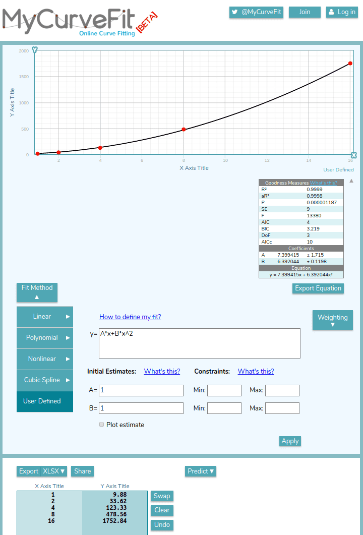
One can use spreadsheet solvers or online curve fitting tools or any other curve fitting software. Just type the pressure versus velocity values from experimental data and let the solver predict \(A\) and \(B\) coefficients. In the above figure, an online tool MyCurveFit \(^1\) is used to predict \(A\) and \(B\) by user defined equation (y=A*x+B*x^2). While y values represent pressure drop, x values represent velocity. In this example, \(A\) and \(B\) coefficients are predicted as 7.4 and 6.4 respectively.
Once \(A\) and \(B\) coefficients are found, extract Darcy \(d\) and Forchheimer \(f\) coefficients from the following equations:
$$d = \frac{A}{\mu \cdot L}$$
$$f = \frac{2B}{\rho \cdot L}$$
References


