What is the Nusselt Number?
The Nusselt number (Nu) is a dimensionless number that represents the ratio of convective to conductive heat transfer across a boundary.
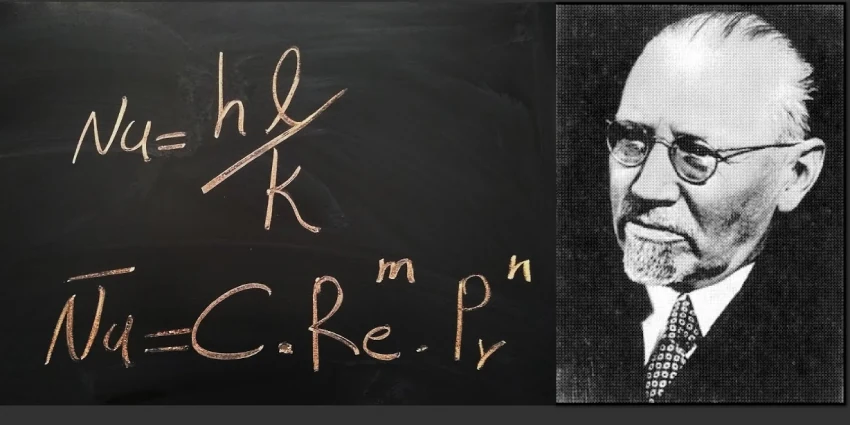
Named after the German engineer Wilhelm Nusselt, it is one of the most important parameters in heat transfer analysis, providing a measure of the enhancement of heat transfer through a fluid layer as a result of convection relative to pure conduction.
In practical terms, the Nusselt number quantifies how effectively a fluid carries heat away from (or toward) a surface. A Nusselt number of 1 indicates that heat transfer occurs purely by conduction through a stagnant fluid layer, while larger values signify increasingly effective convective heat transfer.
The Nusselt number is defined as:
$$ Nu = \frac{hL}{k} \tag{1}$$
where \(h\) \((\frac{W}{m^2 \cdot K})\) is the convective heat transfer coefficient, \(L\) (m) is the characteristic length, and \(k\) \((\frac{W}{m \cdot K})\) is the thermal conductivity of the fluid.
History
Wilhelm Nusselt (1882–1957) was a German engineer who made foundational contributions to the field of heat transfer. Born in Nuremberg, Nusselt studied mechanical engineering at the Technical University of Munich (TUM), where he later became a professor and spent the majority of his academic career.
Nusselt’s most influential work came in 1915, when he published “Das Grundgesetz des Wärmeüberganges” (The Fundamental Law of Heat Transfer), in which he applied dimensional analysis to convective heat transfer problems. In this paper, Nusselt demonstrated that heat transfer between a solid surface and a moving fluid could be described using a dimensionless ratio — what we now call the Nusselt number. This approach was revolutionary because it allowed engineers to generalize experimental heat transfer results across different scales, fluids, and operating conditions.
Nusselt also made important contributions to the understanding of film condensation. His 1916 analysis of the condensation of steam on vertical surfaces — known as the Nusselt film condensation theory — remains a cornerstone of two-phase heat transfer and is still taught in university courses and used in engineering practice today.
The dimensionless number bearing his name was formally adopted by the international scientific community and is now used universally in thermal engineering, computational fluid dynamics (CFD), and heat exchanger design.
Nusselt Number Formula and Derivation
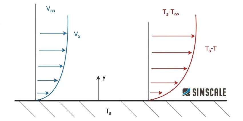
The Nusselt number is derived from the energy balance at a solid-fluid interface. Consider a surface at temperature \(T_s\) in contact with a fluid at temperature \(T_∞\). The heat flux at the wall can be expressed in two equivalent ways:
By convection (Newton’s law of cooling):
$$ q = h(T_s – T_\infty) \tag{2}$$
By conduction through the fluid layer at the wall:
$$ q = -k \frac{\partial T}{\partial y}\bigg|_{y=0} \tag{3}$$
Equating these two expressions and non-dimensionalizing with the characteristic length \(L\):
$$ h = \frac{-k \frac{\partial T}{\partial y}\bigg|_{y=0}}{T_s – T_\infty} \tag{4}$$
$$ Nu = \frac{hL}{k} = \frac{-L \frac{\partial T}{\partial y}\bigg|_{y=0}}{T_s – T_\infty} \tag{5}$$
The Nusselt number is therefore the dimensionless temperature gradient at the surface. A steep temperature gradient (strong convection) yields a high Nu, while a shallow gradient (weak convection, approaching pure conduction) yields Nu approaching 1.
Characteristic Length
The choice of characteristic length \(L\) depends on the geometry:
| Geometry | Characteristic Length \(L\) |
| Internal flow in circular pipe | Pipe diameter \(D\) |
| Internal flow in non-circular duct | Hydraulic diameter \(D_H = \frac{4A}{P}\) |
| External flow over flat plate | Plate length \(x\) (local) or \(L\) (average) |
| External flow over cylinder | Cylinder diameter \(D\) |
| External flow over sphere | Sphere diameter \(D\) |
| Vertical plate (natural convection) | Plate height \(L\) |
Relationship with Other Dimensionless Numbers
The Nusselt number does not exist in isolation — it is typically expressed as a function of other dimensionless numbers that characterize the flow and fluid properties. The most important relationships are:
Reynolds Number
The Reynolds number (Re) represents the ratio of inertial to viscous forces in the flow. In forced convection, the Nusselt number is primarily a function of Re:
$$ Re = \frac{\rho V L}{\mu} = \frac{VL}{\nu} \tag{7}$$
Higher Reynolds numbers correspond to more vigorous fluid mixing, which enhances convective heat transfer and increases the Nusselt number.
Prandtl Number
The Prandtl number (Pr) relates the momentum diffusivity (kinematic viscosity) to the thermal diffusivity of the fluid:
$$ Pr = \frac{\nu}{\alpha} = \frac{\mu c_p}{k} \tag{8}$$
where \(ν\) is the kinematic viscosity, \(α\) is the thermal diffusivity, \(μ\) is the dynamic viscosity, \(c_p\) is the specific heat capacity, and \(k\) is the thermal conductivity. The Prandtl number determines the relative thickness of the velocity and thermal boundary layers. For most forced convection correlations:
$$ Nu = f(Re, Pr) \tag{9}$$
| Fluid | Typical Prandtl Number |
| Liquid metals (e.g., mercury) | 0.01 – 0.03 |
| Gases (e.g., air) | 0.7 – 1.0 |
| Water (at 20°C) | ~7.0 |
| Engine oils | 100 – 40,000 |
Grashof and Rayleigh Numbers
For natural convection, buoyancy-driven flow replaces forced flow, and the Nusselt number depends on the Grashof number (Gr) or the Rayleigh number (Ra):
$$ Gr = \frac{g \beta (T_s – T_\infty) L^3}{\nu^2} \tag{10}$$
$$ Ra = Gr \times Pr = \frac{g \beta (T_s – T_\infty) L^3}{\nu \alpha} \tag{11}$$
where \(g\) is gravitational acceleration, \(β\) is the volumetric thermal expansion coefficient, and \(L\) is the characteristic length. For natural convection:
$$ Nu = f(Ra, Pr) = f(Gr, Pr) \tag{12}$$
Nusselt Number vs. Biot Number
A common point of confusion is the difference between the Nusselt number and the Biot number (Bi). Both have the same mathematical form \(\frac{hL}{k}\), but they differ in the thermal conductivity used:
- Nusselt number: uses the thermal conductivity of the fluid \((k_f)\) — it characterizes heat transfer in the fluid.
- Biot number: uses the thermal conductivity of the solid \((k_s)\) — it characterizes the temperature distribution within the solid.
Nusselt Number Correlations
Nusselt number correlations are empirical or semi-empirical formulas derived from experimental data and theoretical analysis. They allow engineers to calculate the heat transfer coefficient without solving the full Navier-Stokes equations for every new problem.
Forced Convection: Internal Flow
For laminar flow inside a circular tube that is fully developed both hydrodynamically and thermally, the Nusselt number takes constant values depending on the boundary condition:
| Boundary Condition | Nusselt Number |
| Constant wall heat flux | Nu = 4.364 |
| Constant wall temperature | Nu = 3.66 |
These constant values are independent of the Reynolds and Prandtl numbers, which is a distinctive feature of fully developed laminar internal flow.
For turbulent flow in a smooth circular tube, two widely used correlations are:
Dittus-Boelter Equation:
$$ Nu = 0.023 \, Re^{0.8} \, Pr^{n} \tag{13}$$
where \(n = 0.4\) for heating (fluid being heated) and \(n = 0.3\) for cooling (fluid being cooled). This correlation is valid for:
- \(Re > 10{,}000\)
- \(0.6 \leq Pr \leq 160\)
- \(L/D > 10\)
Gnielinski Correlation:
$$ Nu = \frac{(f/8)(Re – 1000) \, Pr}{1 + 12.7 \sqrt{f/8}(Pr^{2/3} – 1)} \tag{14}$$
where \(f\) is the Darcy friction factor. The Gnielinski correlation is considered more accurate than the Dittus-Boelter equation, particularly in the transition region, and is valid for:
- \(2300 \leq Re \leq 5 \times 10^6\)
- \(0.5 \leq Pr \leq 2000\)
Forced Convection: External Flow
Flow over a flat plate (laminar, \(Re_x < 5 \times 10^5\)):
$$ Nu_x = 0.332 \, Re_x^{1/2} \, Pr^{1/3} \quad (Pr > 0.6) \tag{15}$$
Average Nu over the entire plate (laminar):
$$ \overline{Nu}_L = 0.664 \, Re_L^{1/2} \, Pr^{1/3} \tag{16}$$
Flow over a flat plate (turbulent, \(Re_x > 5 \times 10^5\)):
$$ Nu_x = 0.0296 \, Re_x^{4/5} \, Pr^{1/3} \quad (0.6 \leq Pr \leq 60) \tag{17}$$
Flow over a cylinder (Churchill-Bernstein correlation):
$$ \overline{Nu}_D = 0.3 + \frac{0.62 \, Re_D^{1/2} \, Pr^{1/3}}{[1 + (0.4/Pr)^{2/3}]^{1/4}} \left[1 + \left(\frac{Re_D}{282{,}000}\right)^{5/8}\right]^{4/5} \tag{18}$$
Valid for \(Re_D \cdot Pr > 0.2\).
Flow over a sphere (Whitaker correlation):
$$ \overline{Nu}_D = 2 + (0.4 \, Re_D^{1/2} + 0.06 \, Re_D^{2/3}) Pr^{0.4} \left(\frac{\mu}{\mu_s}\right)^{1/4} \tag{19}$$
Valid for \(3.5 \leq Re_D \leq 7.6 \times 10^4\) and \(0.71 \leq Pr \leq 380\).
Note that for a sphere in a stagnant fluid (no convection), \(Nu = 2\), representing pure conduction from a sphere into a surrounding infinite medium.
Natural Convection Correlations
Natural convection correlations depend on the Rayleigh number (Ra) rather than Re. The general form proposed by Churchill and Chu is widely used:
Vertical plate:
$$ \overline{Nu}_L = \left[0.825 + \frac{0.387 \, Ra_L^{1/6}}{[1 + (0.492/Pr)^{9/16}]^{8/27}}\right]^2 \tag{20}$$
Valid for all \(Ra_L\).
Horizontal cylinder:
$$ \overline{Nu}_D = \left[0.60 + \frac{0.387 \, Ra_D^{1/6}}{[1 + (0.559/Pr)^{9/16}]^{8/27}}\right]^2 \tag{21}$$
Valid for \(Ra_D \leq 10^{12}\).
Application: Worked Example
To illustrate how the Nusselt number is used in practice, consider the following scenario: air at 20°C flows over a heated flat plate at 80°C. The plate is 0.5 m long, and the free-stream velocity is 2 m/s. Determine the average heat transfer coefficient.
Given fluid properties of air at the film temperature \((T_f = 50°C)\):
| Property | Value |
| Density \(ρ\) | 1.09 kg/m³ |
| Kinematic viscosity \(ν\) | \(1.798 \times 10^{-5}\) m²/s |
| Thermal conductivity \(k\) | 0.0282 W/(m·K) |
| Prandtl number \(Pr\) | 0.707 |
Step 1 — Calculate the Reynolds number:
$$ Re_L = \frac{VL}{\nu} = \frac{2 \times 0.5}{1.798 \times 10^{-5}} = 55{,}617 \tag{22}$$
Since \(Re_L < 5 \times 10^5\), the flow is laminar over the entire plate.
Step 2 — Calculate the average Nusselt number (Equation 16):
$$ \overline{Nu}_L = 0.664 \times (55{,}617)^{1/2} \times (0.707)^{1/3} = 0.664 \times 235.8 \times 0.891 = 139.5 \tag{23}$$
Step 3 — Calculate the average heat transfer coefficient:
$$ h = \frac{\overline{Nu}_L \times k}{L} = \frac{139.5 \times 0.0282}{0.5} = 7.86 \, \frac{W}{m^2 \cdot K} \tag{24}$$
The average convective heat transfer coefficient for this laminar flow scenario is approximately 7.86 W/(m²·K). Using this value, the total heat transfer rate from the plate can then be calculated using Newton’s law of cooling.
Physical Significance of the Nusselt Number
Understanding what the Nusselt number physically represents helps engineers interpret simulation results and validate their models:
- Nu = 1: Heat transfer is by conduction only (stagnant fluid). This is the theoretical minimum for a single-phase convection problem.
- Nu < 10: Weak convection. Conduction still dominates heat transfer.
- Nu = 10–100: Moderate convection. Typical of many laminar forced convection scenarios.
- Nu > 100: Strong convection. Typical of turbulent flows or flows with significant buoyancy effects.
- Nu > 1000: Very strong convection. Often seen in high-speed turbulent flows or boiling/condensation.
The Nusselt number is especially useful when comparing different heat transfer scenarios — for example, evaluating whether adding fins, increasing flow velocity, or switching fluids will improve cooling performance.
Nusselt Number in SimScale
In SimScale’s Conjugate Heat Transfer (CHT) and Convective Heat Transfer simulations, the Nusselt number is implicitly captured through the resolved temperature and velocity fields. SimScale solves the full Navier-Stokes and energy equations, so the local heat transfer coefficient — and therefore the local Nusselt number — can be extracted from the simulation results as a post-processing step.
Key heat transfer analysis types in SimScale where the Nusselt number is relevant include:
- Conjugate Heat Transfer (CHT): Simultaneously solves fluid flow and solid heat conduction, making it ideal for electronics cooling, heat exchanger design, and thermal management.
- Convective Heat Transfer: Focused on fluid-side heat transfer, useful for validating Nusselt number correlations against full CFD solutions.
- Incompressible Flow with Heat Transfer: For cases where buoyancy effects drive natural convection (using the Boussinesq approximation).
Here are some relevant SimScale resources for exploring heat transfer:
- Conjugate Heat Transfer: Best Practices
- Convective Heat Transfer of a Sphere (Validation)
- Conjugate Heat Transfer in a U-Tube Heat Exchanger (Tutorial)
Frequently Asked Questions
The Nusselt number represents how much more effective convective heat transfer is compared to pure conduction across the same fluid layer. A Nusselt number of 10 means convection transfers heat 10 times more effectively than conduction alone through that fluid.
Both use the formula \(\frac{hL}{k}\), but the Nusselt number uses the thermal conductivity of the fluid while the Biot number uses the thermal conductivity of the solid. The Nusselt number characterizes heat transfer in the fluid; the Biot number characterizes temperature uniformity within the solid.
For a sphere in a stagnant infinite medium, the Nusselt number equals 2, which represents pure radial conduction. For a flat plate with no fluid motion, the Nusselt number approaches 1, representing conduction through a motionless fluid layer. Values below 1 are not physically meaningful in standard single-phase convection.
In forced convection, the Nusselt number increases with the Reynolds number because faster flow produces more vigorous mixing and thinner thermal boundary layers. Most correlations take the form \(Nu = C \cdot Re^m \cdot Pr^n\), where \(m\) is typically between 0.5 (laminar) and 0.8 (turbulent).
For fully developed laminar flow \((Re < 2300)\) in a circular pipe, the Nusselt number is a constant: \(Nu = 4.364\) for constant heat flux and \(Nu = 3.66\) for constant wall temperature. These values are independent of Reynolds and Prandtl numbers.
From CFD simulation results, the Nusselt number can be calculated by extracting the wall heat flux \(q_w\), the wall temperature \(T_w\), and the bulk/free-stream fluid temperature \(T_∞\). First compute \(h = q_w / (T_w – T_∞)\), then \(Nu = hL/k\).
Yes. SimScale AI uses surrogate models and pre-trained foundation models to deliver performance predictions in seconds. You can explore thousands of design variants — varying channel geometries, fin configurations, and flow paths — and shortlist the best candidates before running full-fidelity CFD simulations.
Absolutely. SimScale’s multiphysics capabilities are well-suited for EV battery cold plate design where thermal management, pressure drop optimization, and temperature uniformity across battery cells are all critical. Customers like Rimac Automobili have used SimScale to accelerate electric vehicle battery thermal management development.
References
- Nusselt, W. “Das Grundgesetz des Wärmeüberganges.” Gesundheits-Ingenieur, Vol. 38, 1915, pp. 477–482, 490–496.
- Nusselt, W. “Die Oberflächenkondensation des Wasserdampfes.” Zeitschrift des Vereines Deutscher Ingenieure, Vol. 60, 1916, pp. 541–546, 569–575.
- Incropera, F.P., DeWitt, D.P., Bergman, T.L., and Lavine, A.S. “Fundamentals of Heat and Mass Transfer.” 7th edition. John Wiley & Sons, 2011, ISBN 978-0-470-50197-9. [Link]
- Cengel, Y.A. and Ghajar, A.J. “Heat and Mass Transfer: Fundamentals and Applications.” 5th edition. McGraw-Hill, 2015, ISBN 978-0-07-339818-1. [Link]
- White, F.M. “Fluid Mechanics.” 4th edition. McGraw-Hill, 2002, ISBN 0-07-228192-8. [Link]
- Churchill, S.W. and Bernstein, M. “A Correlating Equation for Forced Convection From Gases and Liquids to a Circular Cylinder in Crossflow.” Journal of Heat Transfer, Vol. 99, 1977, pp. 300–306. [Link]
- Churchill, S.W. and Chu, H.H.S. “Correlating Equations for Laminar and Turbulent Free Convection from a Vertical Plate.” International Journal of Heat and Mass Transfer, Vol. 18, 1975, pp. 1323–1329. [Link]
Last updated: March 16th, 2026
Did this article solve your issue?
How can we do better?
We appreciate and value your feedback.
What's Next
What Are Boundary Conditions?

