Documentation
Convection is the transfer of heat from solid to fluid or vice versa depending upon the temperature. This transfer of heat is brought about by the bulk movement of the fluid. The faster the flow, the higher the heat transfer. However, it also depends on the temperature difference between the solid and the bulk fluid. Despite the complexity of the nature of convection it is normal to express convection using conventional Newton’s law of heating/cooling as follows:
$$Q=hA_s\left(T_0-T_\infty\right)$$
where h is the convective heat transfer coefficient and As is the surface area available for heat transfer.
All the complexity associated with convection is now captured by the heat transfer coefficient. Now the problem becomes determining an analytical expression for the heat transfer coefficient. Although the coefficient looks simple, it really isn’t. The heat transfer coefficient captures a lot of physical phenomena. Therefore, the heat transfer coefficient depends on a lot of parameters for the heat transfer scenario. Some of the parameters which affect the value of the convection coefficient are as follows:
Convection can be forced where the fluid is being moved by an external source like a fan, pump, or wind, and the bulk fluid velocity is approximately constant.
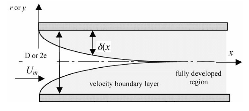
As we know, whenever a fluid flows over a solid surface under equilibrium, a boundary layer is developed. A boundary layer is a fluid region of low momentum. The velocity of the flow very close to the solid boundary at y → 0 is 0. Essentially the fluid is stationary where it contacts the solid surface. The flow speed slowly increases as we go further away from the solid surface to eventually match the bulk fluid flow speed.

So actually speaking, close to the boundary the heat transfer happens due to conduction through the liquid as the liquid is not moving at y → 0.
$$Q=-kA_s\left(\frac{\partial T}{\partial y}\right)_{y=0}$$
Equating the conduction heat transfer to convective heat transfer gives:
$$h=-\frac{k\left(\frac{\partial T}{\partial y}\right)_{y=0}}{\left(T_0-T_\infty\right)}$$
where k is thermal conductivity.
The total temperature difference between the solid surface and the bulk fluid will be \(\left(T_0-T_\infty\right)=\Delta T\). Within the thermal boundary layer with a very small thickness of \(\delta_T\) and a total temperature change of \(\Delta T\), the convective heat transfer coefficient can be written as:
$$h=-\frac{k\left(\frac{\Delta T}{\delta_T}\right)}{\Delta T}=\frac{-k}{\delta_T}$$
For defining the flow field we can start from the mass and momentum conservation equations assuming a 2D flow field which are as follows:
$$\frac{\partial u}{\partial x}+\frac{\partial v}{\partial y}=0$$
$$u \frac{\partial u}{\partial x} + v \frac{\partial u}{\partial y} = – \left(\frac{1}{\rho}\right) \left(\frac{\partial P}{\partial x}\right) + \nu \left(\frac{\partial^2 u}{\partial x^2} + \frac{\partial^2 u}{\partial y^2}\right)$$
$$u \frac{\partial v}{\partial x} + v \frac{\partial v}{\partial y} = – \left(\frac{1}{\rho}\right) \left(\frac{\partial P}{\partial y}\right) + \nu \left(\frac{\partial^2 v}{\partial x^2} + \frac{\partial^2 v}{\partial y^2}\right)$$
$$u \frac{\partial T}{\partial x} + v \frac{\partial T}{\partial y} = \alpha \left(\frac{\partial^2 T}{\partial x^2} + \frac{\partial^2 T}{\partial y^2}\right)$$
where,
u = fluid velocity in the x direction
v = fluid velocity in the y direction
\(\nu\) = kinematic viscosity
\(\alpha\) = thermal diffusivity
k = thermal conductivity
From the equation of continuity and momentum with an order of magnitude analysis, the following can be obtained:
$$\frac{U_\infty}{L}=\frac{v}{\delta}$$
where,
\(\delta\) = boundary layer thickness
L = length of the solid surface
\(U_\infty\) = free stream velocity
v = velocity of the flow perpendicular to the surface
The following shows the different terms of momentum equations. The first two are the momentum terms, the third one is the pressure term, and the last two terms are flow friction terms.
$$\frac{{U_\infty}^2}{L},\frac{v U_\infty}{\delta},\frac{P}{\rho L},\nu \frac{U_\infty}{L^2}, \nu \frac{U_\infty}{\delta^2}$$
It can be easily seen that the 4th term, which is a flow friction term, is much smaller than the last term and can be neglected for both momentum equations. Therefore,
\(\frac{\partial^2}{\partial x^2}\) can be safely dropped.
Similarly, for the pressure term for both the x and y momentum equations, the pressure gradient should balance the flow friction term, then an order of the magnitude of different pressure gradient will be as follows:
$$\left(\frac{1}{\rho}\right)\left(\frac{\partial P}{\partial x}\right)\sim \nu \frac{\partial^2 u}{\partial y^2} \text{ and } \left(\frac{1}{\rho}\right)\left(\frac{\partial P}{\partial y}\right)\sim \nu \frac{\partial^2 v}{\partial y^2}$$
$$\frac{\partial P}{\partial x} \sim \mu\frac{U_\infty}{L^2} \text{ and } \frac{\partial P}{\partial y} \sim \mu\frac{v}{\delta^2}$$
Clearly, the pressure gradient in y is negligible as compared to the pressure gradient in x and as such the pressure gradient within the boundary layer will be the same as the pressure gradient within the bulk flow. By equating the inertia term with the friction term the following relationship is obtained:
$$\frac{{U_\infty}^2}{L} = \nu\frac{U_\infty}{\delta^2} \Rightarrow \delta = \left(\frac{\nu L}{U_\infty}\right)^\frac{1}{2} \Rightarrow \frac{\delta}{L} = {{Re}_L}^{-\frac{1}{2}}$$
where ReL is Reynold’s number \(=\frac{U_\infty}{\nu L}\)
Similarly, using the order of magnitude analysis for the energy equation the following terms are obtained:
$$\frac{U_\infty \Delta T}{L} , \frac{v\Delta T}{\delta_T} , \alpha\frac{\Delta T}{L^2} , \alpha\frac{\Delta T}{{\delta_T}^2}$$
Again the 3rd term is negligible as compared to the 4th one as \(L\text{ >> }{\delta_T}^2\). Then equating the term results in the following relationship:
$$\frac{v\Delta T}{\delta_T} \sim \frac{U_\infty \Delta T}{L}\left(\frac{\delta}{\delta_T}\right)$$
If the thermal boundary layer is much thicker than the velocity boundary layer, i.e. \(\delta\text{ << }\delta_T\), it would imply that the second term in the energy equation will be small as compared to the first term and can therefore be dropped. The equation then comes out to be:
$$\frac{U_\infty \Delta T}{L} \sim \alpha\frac{\Delta T}{{\delta_T}^2} \Rightarrow \frac{\delta_T}{L} \sim {Pr}^{-\frac{1}{2}} {{Re}_L}^{-\frac{1}{2}} \Rightarrow \frac{\delta_T}{\delta} \sim Pr^{-\frac{1}{2}}$$
where Pr is Prandtl number \(\frac{\nu}{\alpha}\)
From the above equation, we can conclude that if \(\delta << \delta_T, Pr < 1\) (this range is generally denoted by liquid metals) then the convective heat transfer coefficient can be written as:
where Nu is Nusselt number \(=\frac{hL}{k}\)
If the thermal boundary layer is smaller than the velocity boundary layer \(\delta >> \delta_T\), then the term u will be \(U_\infty \frac{\delta_T}{\delta}\) and due to mass conservation \(\frac{u}{L} = \frac{v}{\delta_T}\). Using all of these, the following relation can be derived:
$$\frac{\delta_T}{L} \sim {Pr}^{-\frac{1}{3}} {{Re}_L}^{-\frac{1}{2}} \Rightarrow \frac{\delta_T}{\delta} \sim {Pr}^{-\frac{1}{3}} \Rightarrow h \sim \frac{k}{L} {Pr}^{\frac{1}{3}} {{Re}_L}^{\frac{1}{2}} \Rightarrow \text{Nu} \sim {Pr}^{\frac{1}{3}} {{Re}_L}^{\frac{1}{2}}$$
From the above equation, it can be obtained that Pr < 1 since \(\delta >> \delta_T\). All the above relations are valid for a forced convention flow over a flat plate with constant solid surface temperature.
In this section, a list of some of the expressions of convective heat transfer coefficients/Nusselt numbers are listed that can be used as a first approximation for analytical calculations:
The value of a Nusselt number can be different depending on the analytical method used to derive it. The most commonly used methods are scaling, integral, and similarity solutions. Using similarity solutions, the average Nusselt number comes out to be as follows. All these results are valid for flat isothermal plates with laminar flow, i.e. for \(Re < 5 (10^5)\).
$$Nu = 1.128 {Pr}^\frac{1}{2} {{Re}_L}^\frac{1}{2} \text{for Pr } < 0.5$$
$$Nu = 0.664 {Pr}^\frac{1}{3} {{Re}_L}^\frac{1}{2} \text{for Pr } > 0.5$$
For the complete range of Pr number the following expression can also be used:
$$Nu = \frac{0.928 {Pr}^\frac{1}{3} {{Re}_L}^\frac{1}{2}}{\left(1+\left(\frac{0.0207}{Pr}\right)^\frac{2}{3} \right)^\frac{1}{4}}$$
The local Nusselt number comes out to be:
$${Nu}_x = 0.564 {Pr}^\frac{1}{2} {{Re}_x}^\frac{1}{2} \text{for Pr } < 0.5$$
$${Nu}_x = 0.322 {Pr}^\frac{1}{3} {{Re}_x}^\frac{1}{2} \text{for Pr } > 0.5$$
For plates with unheated starting section of \(x = x_0 \text{for Pr } > 0.5\)
$${Nu}_x = 0.322 {Pr}^\frac{1}{3} {{Re}_x}^\frac{1}{2} \left(1-\left(\frac{x_0}{x}\right)^\frac{3}{4}\right)^{-\frac{1}{3}}$$
If the wall heat flux is constant instead of the wall temperature then the following expression for Nusselt number can be used for 10 > Pr > 0.5:
$${Nu}_x = 0.453 {Pr}^\frac{1}{3} {{Re}_x}^\frac{1}{2}$$
| Geometry | Thermal Conditions | Nu |
| Cylindrical duct | Uniform wall heat flux | 4.36 |
| Cylindrical duct | Uniform wall temperature | 3.66 |
| Plane channel | Uniform wall heat flux | 8.23 |
| Plane channel | Uniform wall temperature | 7.54 |
Here, the Reynolds number is calculated based on hydraulic diameter. The diameter can be calculated as follows:
$$D_h = \frac{4S}{P}$$
where,
S = cross section area
P = wetted perimeter
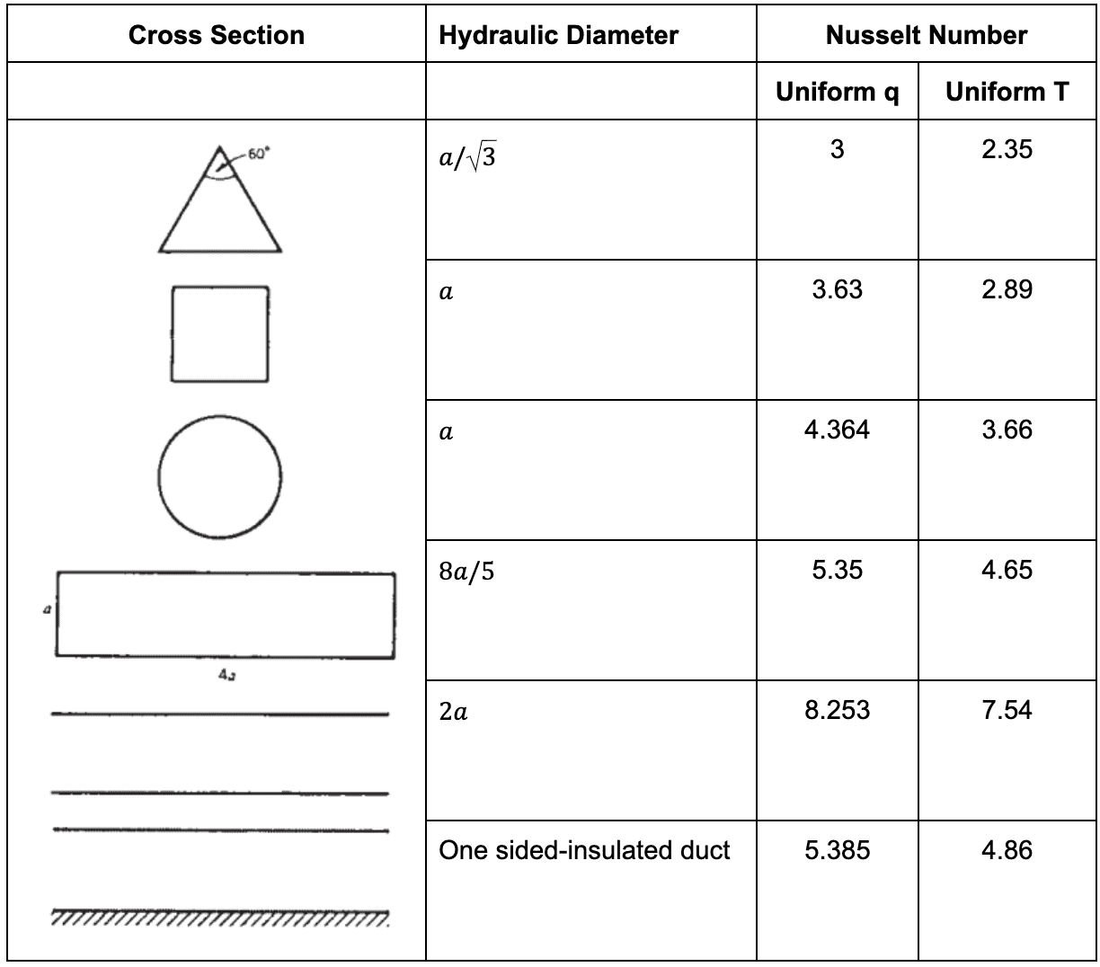
Some additional Nusselt numbers for ducts with different cross-sections for uniform, laminar flows are as follows:
For flow past a wedge, where a longitudinal pressure difference is present and the wall is isothermal, the following values for local Nusselt number applies:
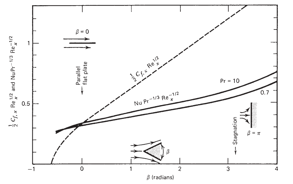
The table below shows the value of \(\frac{Nu}{{{Re}_x}^\frac{1}{2}}\) for different wedge angles and Prandtl numbers, which in turn could be used for computing the local convective heat transfer coefficient.
The average heat transfer coefficient is derived from the local heat transfer coefficient with the following relationship:
$$h_{avg} = \frac{2h}{1+m}$$
| \(\boldsymbol{\beta}\) | m | Pr 0.7 | Pr 0.8 | Pr 1 | Pr 5 | Pr 10 |
| -0.512 | -0.0753 | 0.242 | 0.253 | 0.272 | 0.457 | 0.570 |
| 0 | 0 | 0.292 | 0.307 | 0.332 | 0.585 | 0.730 |
| \(\frac{\pi}{5}\) | \(\frac{1}{9}\) | 0.331 | 0.348 | 0.378 | 0.669 | 0.851 |
| \(\frac{\pi}{2}\) | \(\frac{1}{3}\) | 0.384 | 0.403 | 0.440 | 0.792 | 1.013 |
| \(\pi\) | 1 | 0.496 | 0.523 | 0.570 | 1.043 | 1.344 |
| \(\frac{8\pi}{5}\) | 4 | 0.813 | 0.858 | 0.938 | 1.736 | 2.236 |
The following is a scale analysis of a 2D surface of length H vertically oriented and the gravity g acting along perpendicular to the normal of the 2D surface in -y direction. Using a similar logic to the one used for forced convection, the following equations for momentum and thermal energy within the boundary layer can be obtained. Note that, unlike the forced convection case, here the boundary layer is developing along the y-axis as such \(\delta_T << H\) and a result of this is that the \(\frac{\partial^2 T}{{\partial y}^2}\) becomes much smaller in comparison to \(\frac{\partial^2 T}{{\partial x}^2}\).
$$u \frac{\partial T}{\partial x} + v \frac{\partial T}{\partial y} = \alpha \left(\frac{\partial^2 T}{\partial x^2}\right)$$
$$\rho \left(u \frac{\partial v}{\partial x} + v \frac{\partial v}{\partial y}\right) = – \frac{{\Delta P}_\infty}{\Delta y} + \mu \left(\frac{\partial^2 v}{\partial x^2}\right) – \rho g$$
$$\rho \left(u \frac{\partial v}{\partial x} + v \frac{\partial v}{\partial y}\right) = \mu \left(\frac{\partial^2 v}{\partial x^2}\right) + \left(\rho_\infty – \rho\right)g$$
This equation can again be rewritten in terms of volume expansion coefficient \(\beta\) as follows:
$$\rho \left(u \frac{\partial v}{\partial x} + v \frac{\partial v}{\partial y}\right) = \mu \left(\frac{\partial^2 v}{\partial x^2}\right) + \beta \left(T – T_\infty\right)g$$
The scale analysis for the energy equation comes to be as follows:
$$\frac{u\Delta T}{\delta_T} , \frac{v\Delta T}{H} \sim \alpha \frac{\Delta T}{{\delta_T}^2}$$
From continuity equations the following relationship still holds:
$$\frac{u}{\delta_T} \sim \frac{v}{H}$$
Using the above two equations, the following relation can be obtained:
$$v \sim \alpha \frac{H}{{\delta_T}^2}$$
The order of magnitude of the terms of the equation of momentum are as follows:
$$\frac{vu}{\delta_T} , \frac{v^2}{H} , \nu \frac{v}{{\delta_T}^2} , g\beta \Delta T$$
In terms of dimensionless quantities like Prandtl number and Rayleigh number, the following expression can be obtained:
$$\left(\frac{H}{\delta_T}\right)^4 {{Ra}_H}^{-1 }{{Pr}^{-1}} , \left(\frac{H}{\delta_T}\right)^4 {{Ra}_H}^{-1} , 1 $$
Where Rayleigh number is defined as:
$${Ra}_H = \frac{{g \beta \Delta TH}^3}{\alpha \nu}$$
When \(Pr >> 1\) there is a balance between buoyancy and friction:
$$\text{Nu} = \frac{hH}{k} \sim {{Ra}_H}^\frac{1}{4}$$
If \(Pr << 1\), there is a balance between buoyancy and inertia, and the following relationship between Nu can be obtained:
$$\text{Nu} = \frac{hH}{k} \sim \left({Ra}_H \cdot Pr\right)^\frac{1}{4}$$
The integral solution result for natural convection past a vertical isothermal plate comes out to be:
$$\text{Nu} = 0.783 {{Ra}_y}^\frac{1}{4} \text{ and Nu } = 0.689 \left({Ra}_y \cdot Pr\right)^\frac{1}{4}$$
For \(Pr >> 1\) and \(Pr << 1\) respectively, and by using the similarity solution, the result comes out to be:
$$\text{Nu} = 0.503 {{Ra}_y}^\frac{1}{4} \text{ and Nu } = 0.6 \left({Ra}_y \cdot Pr\right)^\frac{1}{4}$$
The value of average Nu comes out to be:
$$\text{Nu} = 0.671 {{Ra}_H}^\frac{1}{4} \text{ and Nu } = 0.8 \left({Ra}_H \cdot Pr\right)^\frac{1}{4}$$
For the constant flux case, the values of Nusselt numbers are as follows:
$$\text{Nu} = \frac{2}{{360}^\frac{1}{5}} \left(\frac{Pr}{\frac{4}{5} + Pr}\right)^\frac{1}{5} {{Ra}_{*y}}^\frac{1}{5}$$
Here Rayleigh number is defined differently as follows:
$${Ra}_H = \frac{{g \beta H}^4 q”}{\alpha \nu k}$$
where,
q” = heat flux
k = thermal conductivity
y = length of the vertical plate from point of start of thermal boundary layer
For turbulent flows, the expressions for average Nusselt number are as follows:
$${Nu}_H = \left(0.825 + \frac{0.387{{Ra}_H}^\frac{1}{6}}{\left(1 + \left(\frac{0.492}{Pr}\right)^\frac{9}{16}\right)^\frac{8}{27}}\right)^2$$
Here, the Rayleigh and Prandtl numbers are calculated for the average of wall and flow temperature. For a case with constant heat flux and turbulent flow conditions, the Nusselt number is calculated as follows:
$$\text{Nu } = 0.645 {{Ra}_{*H}}^{0.22}$$
For inclined walls, the expression for Nusselt number remains unchanged and the effect of inclination is accounted for in the Rayleigh number as follows:
$${Ra}_H = \frac{cos\left(\phi \right)g \beta H^4 q”}{\alpha \nu k} \text{ and } {Ra}_H = \frac{cos\left(\phi \right)g \beta \Delta T H^3}{\alpha \nu}$$
where \(\phi\) is the angle of the wall surface with respect to the direction of gravity.
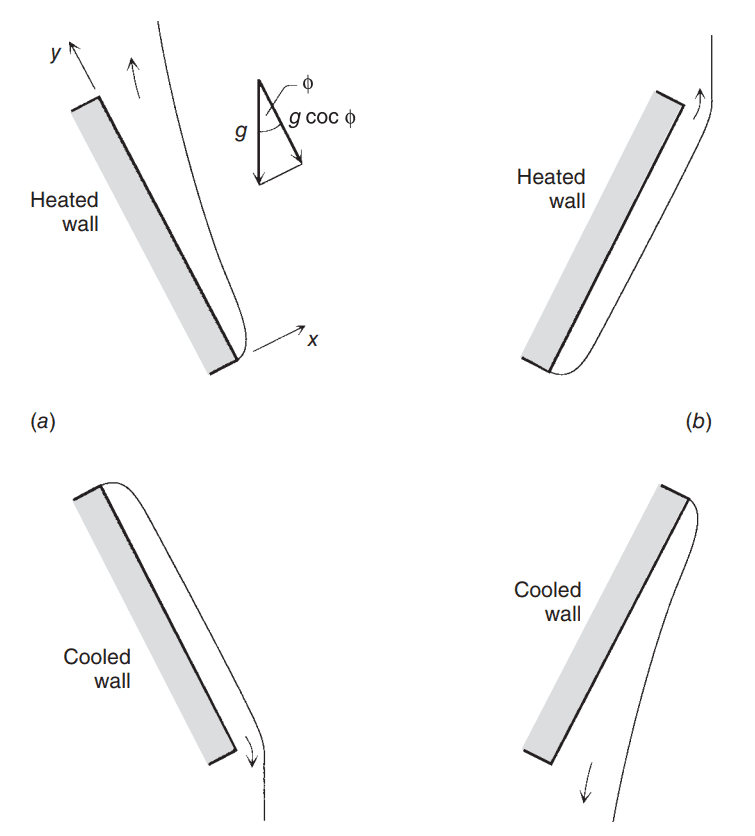
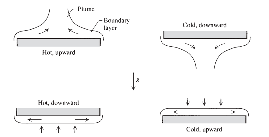
The value of Nusselt number for hot surfaces facing upwards or cold surface facing downwards is as follows:
$$Nu = 0.54 {{Ra}_H}^\frac{1}{4} \text{ for } \left({10}^4 < {Ra}_H < {10}^7\right)$$
$$Nu = 0.15 {{Ra}_H}^\frac{1}{3} \text{ for } \left({10}^7 < {Ra}_H < {10}^9\right)$$
For hot surfaces facing downwards and cold surfaces facing upwards, the expression for Nusselt number is as follows:
$$Nu = 0.27 {{Ra}_H}^\frac{1}{4} \text{ for } \left({10}^5 < {Ra}_H < {10}^{10}\right)$$
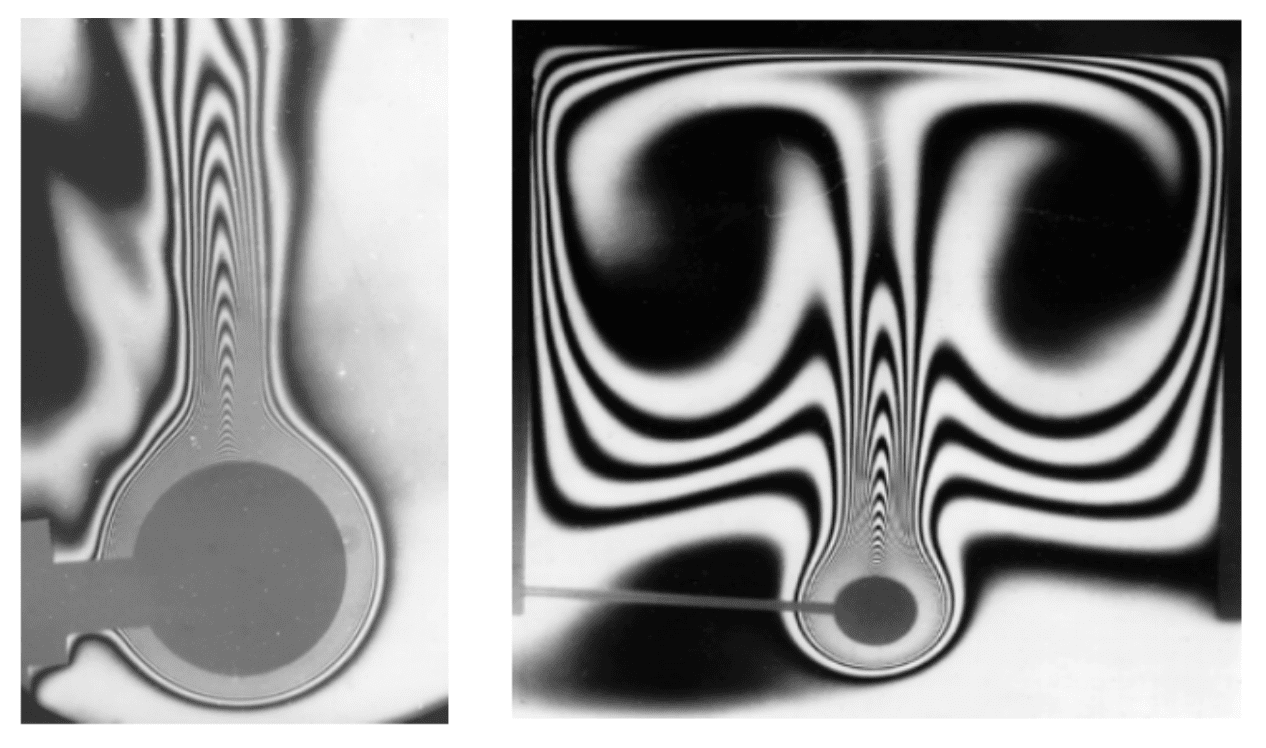
For a horizontal isothermal cylinder with the axis of rotation perpendicular to the direction of gravity the Nusselt number is as follows:
$${Nu}_D = \left(0.6 + \frac{0.387{{Ra}_D}^\frac{1}{6}}{\left(1 + \left(\frac{0.599}{Pr}\right)^\frac{9}{16}\right)^\frac{8}{27}}\right)^2$$
where, \({Nu}_D = \frac{hD}{k} \text{ and } {Ra}_D = \frac{g \beta \Delta T D^3}{\alpha \nu}\).
For an isothermal vertical cylinder the expression for Nusselt number is as follows:
$${Nu}_H = \frac{4}{3} \left(\frac{7{Ra}_{H}Pr}{5\left(20 + 21Pr\right)}\right)^\frac{1}{4} + \frac{4\left(272 + 315Pr\right)H}{35\left(64 + 63Pr\right)D}$$
For an isothermal sphere the expression is as follows:
$${Nu}_D = \left(2 + \frac{0.589 {{Ra}_D}^\frac{1}{4}}{\left(1 + \left(\frac{0.469}{Pr}\right)^\frac{9}{16}\right)^\frac{4}{9}}\right)$$
for \(Pr > 0.7 \text{ and } {Ra}_D < 10^{11}\)
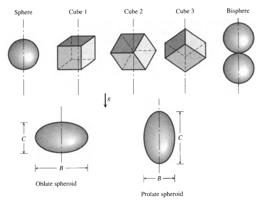
For an isothermal body of any shape the length is defined as follows:
$$\gamma = A^\frac{1}{2}$$
where A is the surface area of the body in contract with the fluid.
The above mentioned length scale is used for both Nusselt number and Rayleigh number:
$${Nu}_\gamma = \left({{Nu}_\gamma}^0 + \frac{{0.67G_\gamma {Ra}_\gamma}^\frac{1}{4}}{\left(1 + \left(\frac{0.492}{Pr}\right)^\frac{9}{16}\right)^\frac{4}{9}}\right)$$
where the values of \({{Nu}_\gamma}^0 \) and \(G_\gamma\) can be obtained from the table below:
| Body Shape | \(\boldsymbol{{Nu}_\gamma}^0\) | \(\boldsymbol G_\gamma\) |
| Sphere | 3.545 | 1.023 |
| Bi-sphere | 3.475 | 0.928 |
| Cube 1 | 3.338 | 0.951 |
| Cube 2 | 3.338 | 0.990 |
| Cube 3 | 3.338 | 1.014 |
| Vertical short cylinder (L~D) | 3.444 | 0.967 |
| Horizontal short cylinder | 3.444 | 1.019 |
| Short cylinder at 45° | 3.444 | 1.004 |
| Prolate spheroid (\(\frac{C}{B} = 1.93\)) | 3.566 | 1.012 |
| Oblate spheroid (\(\frac{C}{B} = 0.5\)) | 3.529 | 0.973 |
| Oblate spheroid (\(\frac{C}{B} = 0.1\)) | 3.342 | 0.768 |
For plates with a small spacing between them, i.e. the spacing between the plates is smaller than the thermal boundary layer, the total heat transfer rate can be computed as follows:
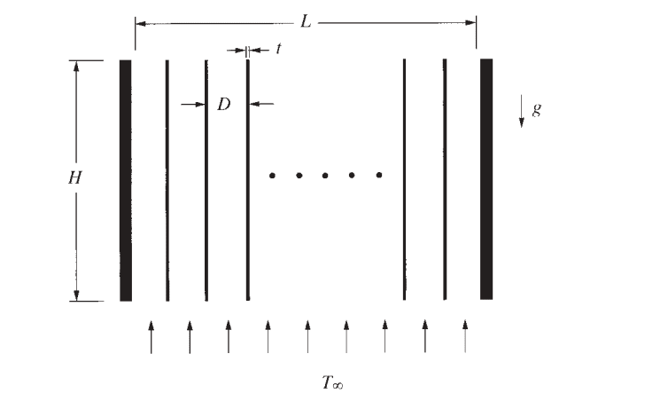
$$q_A = \frac{\rho g \beta C p \left(\Delta T\right)^2 D^3}{12 \nu} W \frac{L}{D}$$
where W is the width of the plates perpendicular to the figure plane.
If the spacing between the plates is sufficiently larger \(D > {H{Ra}_H}^{-\frac{1}{4}}\) than the thickness of the boundary layer formed, then the expressing for heat transfer is as follows:
$$q_A = 2 \frac{k}{H} W H \Delta T \frac{L}{D} 0.516{{Ra}_H}^\frac{1}{4}$$
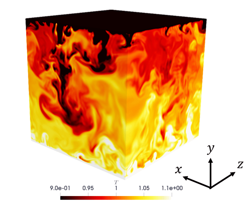
Computational Fluid Dynamics (CFD) can be used to study convection at many different scales and for different problems. For example, CFD can be used in the academic understanding of the flow patterns occurring in convection, using LES or DNS simulations, and understanding large industrial scale problems using RANS simulations.
In CFD, convection occurs where there are temperature differences and when either a gravitational direction is specified (Natural Convection) or there is a defined flow (Forced Convection). Temperature gradients can be set in a variety of different ways. It is important to note, a solver that incorporates the energy equation is necessary here. Incompressible, isothermal solvers are not suitable for these types of studies.
A boundary condition is where we define all the things we know about a problem on the boundary surfaces of a flow domain. In convective CFD simulations, this might be a fixed temperature, or it could be a power, heat flux, or heat transfer coefficient. Usually, this will create a temperature gradient and the CFD will calculate the flow patterns as discussed in previous sections.
Volumetric sources usually defined as a power or a volumetric power (per cubic meter) are a good way of modeling some internal sources. For example, in an office room, people and equipment emit heat. However, they are not always static, and instead, we might want to model them more arbitrarily as a volume source, saying that the volume represents 10 people dynamically moving in the space.
Natural convection is buoyancy-driven, i.e. as the air heats up, its density is reduced and thus moves in a direction opposite to gravity. In this sense, it is important to correctly orient the model and define gravity and its strength. In most cases, gravity is \(-9.81 \frac{m}{s^2}\) in the z-direction. However, caution should be taken to ensure that the model is correctly oriented to this axis. If a flow is strongly forced convection, gravity need not be defined. However, there are many scenarios where buoyancy plays a strong role in some parts of a CFD simulation and not others. Therefore, it may be interesting to test study this for your specific application.
Convection, both natural and forced, is regularly simulated by SimScale customers and users. In this section, we will be discussing these uses in the AEC and electronic cooling industries.
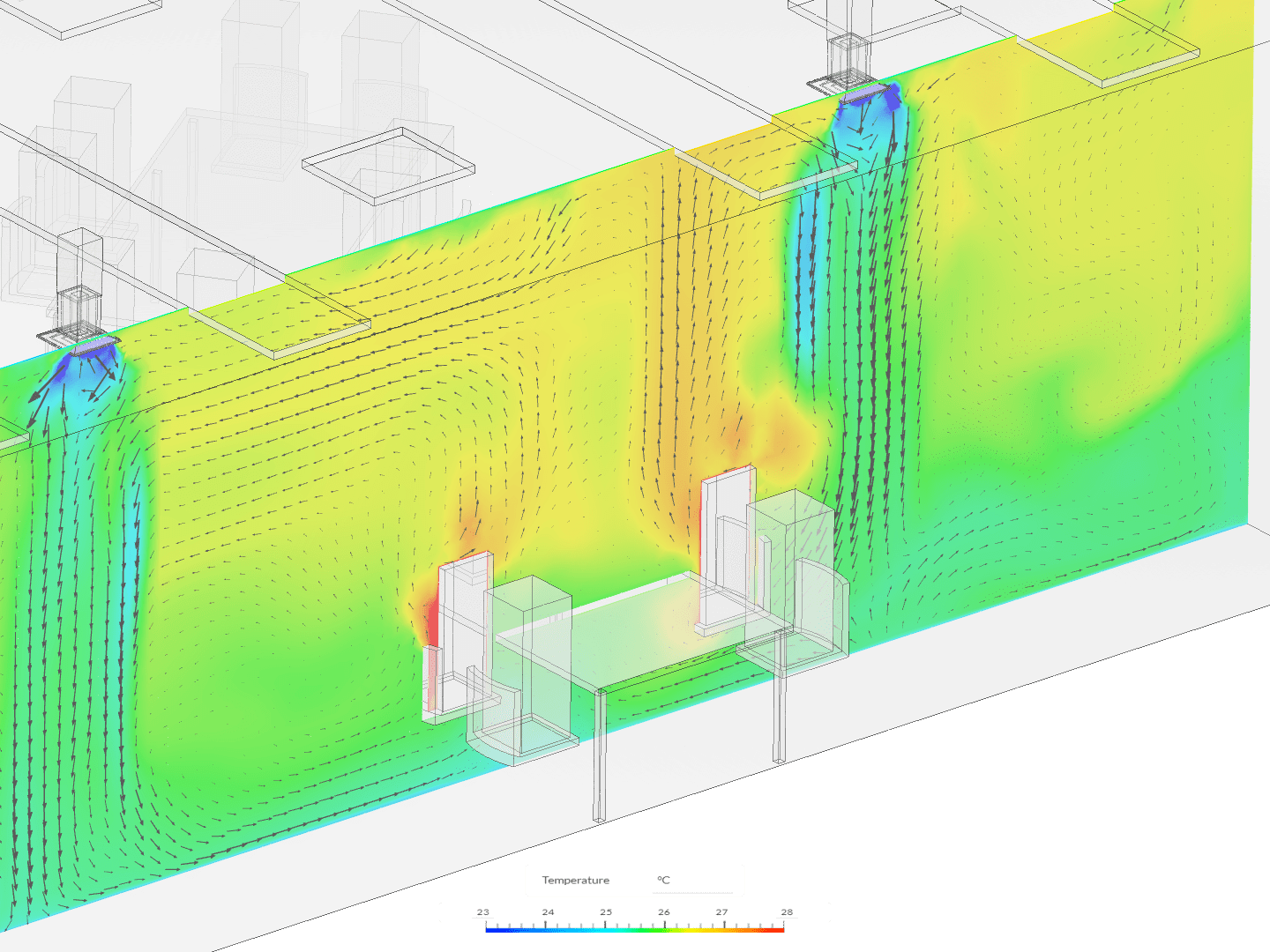
In the AEC industry, the act of heating a room with heaters, or simply heat convecting off of people and occupants within a room, is convection. The act of cooling the spaces down by opening windows or with HVAC equipment are examples of convection. The AEC industry drastically influences global energy consumption and therefore a detailed understanding of these sometimes complex convective flows is becoming increasingly important.
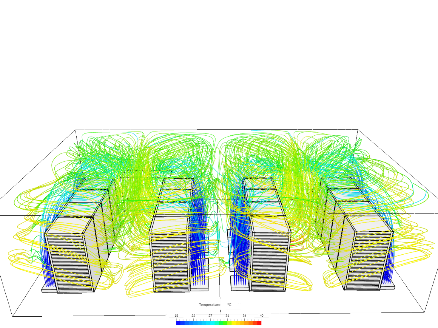
Meanwhile, in electronics cooling, hot components (LEDs, embedded circuits, battery cells, etc.) either in enclosures or open-to-ambient conditions are both natural convection scenarios. If we add fans, blowers, and pumps to the design, they can also incorporate forced convection. Electronics are being embedded into more and more devices, becoming more complex, and ever more important to everyday life. The increased ‘intelligence’ of many important systems is a useful tool to help combat the contributors to global warming. Therefore, understanding convection around these devices can have significant impacts on the above-mentioned issues.
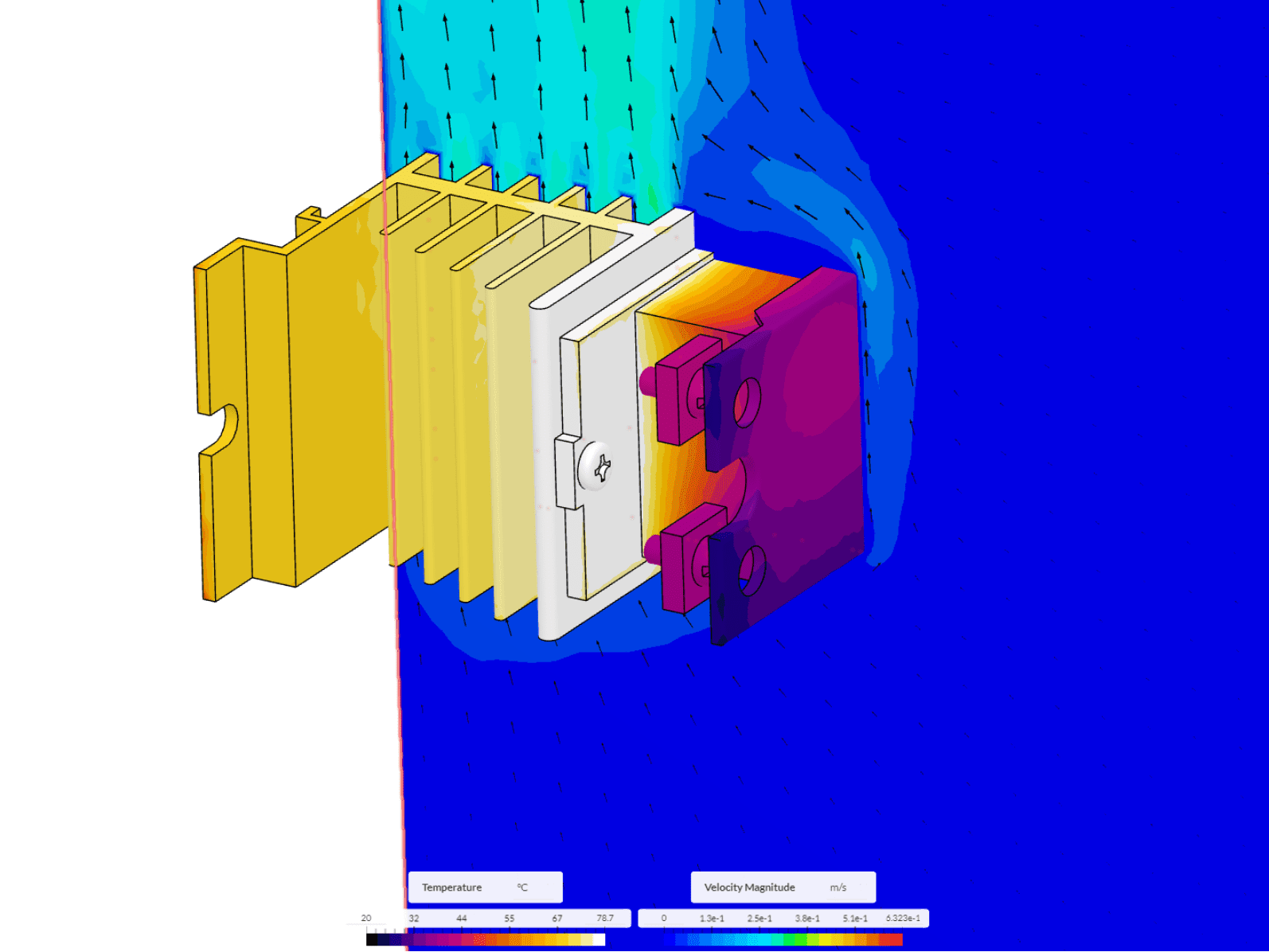
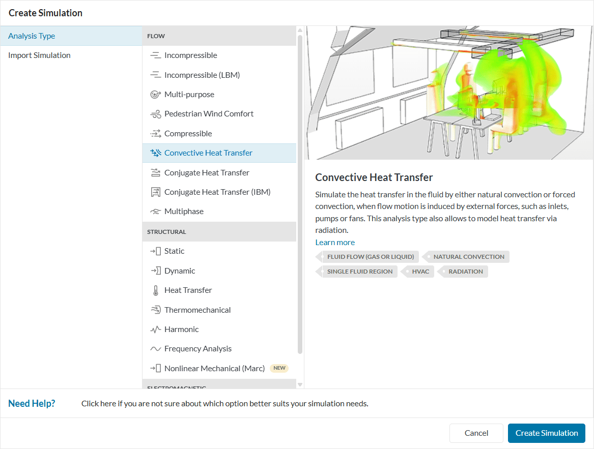
Convection can happen whenever there is a fluid involved and there is a temperature difference. In reality, this is almost every real fluid flow. However, in CFD we simplify our models as much as possible, and reserve temperature difference-driven flows to a set of simulation types. In SimScale, convection can be solved using the listed current solvers:
Conjugate Heat Transfer is available in two forms, CHT and CHT (IBM). CHT is based on so-called body-fitted meshes, where the meshing algorithm stays conformal with the geometrical boundaries of the geometry. CHT (IBM) is based on the Immersed Boundary Method and immerses the geometry into a cartesian background grid.
Conjugate Heat Transfer allows us to model the three main heat transfer modes (convection, conduction, and radiation) allowing us to apply solid and fluid materials to our simulation models. This is particularly useful when multiple fluid voids interact through solid parts. This is mainly used for electronic cooling applications, but also finds its way into many other applications.
Conjugate Heat Transfer is also able to operate in convection, conduction and/or radiation-only mode if no solids or fluids respectively are assigned materials. It will therefore one day also supersede the Convective Heat Transfer analysis type.
Convective Heat Transfer has been one of our most used solvers, seeing most of its use for AEC applications such as room-level thermal comfort and air quality problems. Its diversity and robustness allow quick analysis of room HVAC layouts and provides valuable feedback on what can be improved before too much time is invested. As mentioned before, it will eventually be superseded by CHT, as that solver adds speed and stability to the mix.
Multi-purpose analysis type
Convective heat transfer simulations can also be performed in SimScale’s Multi-purpose analysis type.
SimScale has some great tutorials and projects to get started with industrial convection cases, here are some of our favorites:
You can sign up for a SimScale account anytime using this link. Happy Simulation!
References
Last updated: March 16th, 2026
We appreciate and value your feedback.
What's Next
Numerics Background for CFD and FEASign up for SimScale
and start simulating now