Tutorial: Conjugate Heat Transfer in a U-Tube Heat Exchanger

This tutorial shows how a conjugate heat transfer simulation in a U-tube heat exchanger can be performed using SimScale’s CHT v2 solver.

This kind of heat exchanger is named after the U-shaped tube and is a simple, low price structure with less sealing surface. It has a tube configuration that can expand or contract freely, without producing thermal stress due to the temperature difference between the tube and shell, leading to a good thermal compensation performance. SimScale can simulate and visualize this thermal conduction between the solid shell and the two streams that flow within.

Overview

This tutorial teaches users how to:

• Set up and run a conjugate heat transfer simulation using CHT v2 solver.
• Assign boundary conditions, material assignments, and other properties to the simulation.
• Mesh with SimScale’s standard meshing algorithm.
• Post-process the results in SimScale.

You are following the typical SimScale workflow:

1. Prepare the CAD model for the simulation.
2. Set up the simulation.
3. Create the mesh.
4. Run the simulation and analyze the results.

1. Prepare the CAD Model and Select the Analysis Type

1.1. Import the CAD into Your Workbench

First of all, click the button below.

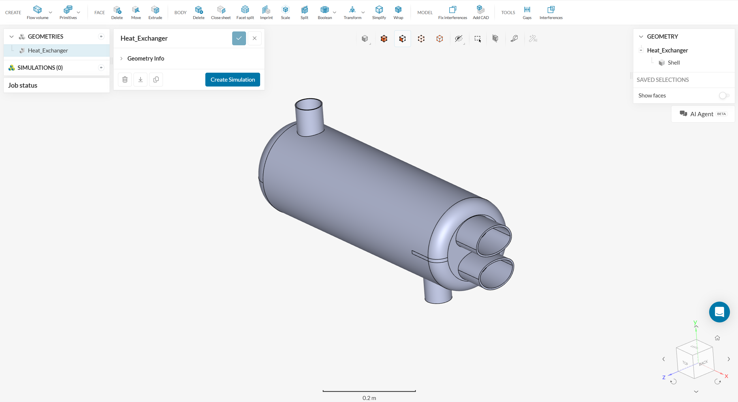
The following picture demonstrates what should be visible after importing the u-tube heat exchanger tutorial project.

1.2. CAD Mode

Before you start setting up the u-tube heat exchanger simulation, you need to do some CAD pre-processing. As you simulate a conjugate heat transfer, you want to know the heat transfer between solids and fluids. Natively you already have the solid shell CAD part, now you need to create the flow regions.
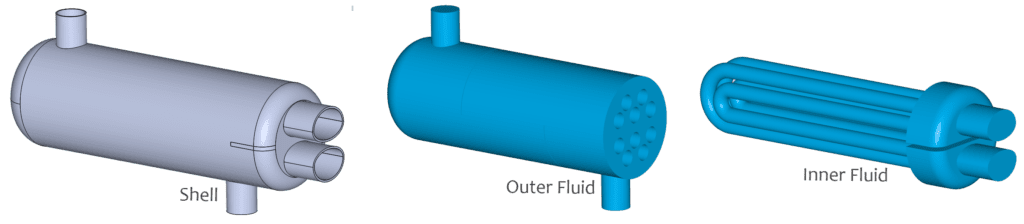
The following picture illustrates the parts you need for setting up the simulation:

Finally, you need to run an Imprint operation to enhance the automatic contact detection. All of these steps are possible within SimScale’s CAD Mode:

a. Open Inner Region for Modelling the Inner Region

In CAD Mode, the first step is the creation of an Internal Flow Volume operation. In this step, you will assign a Seed face, as well as the boundary faces of the flow region.

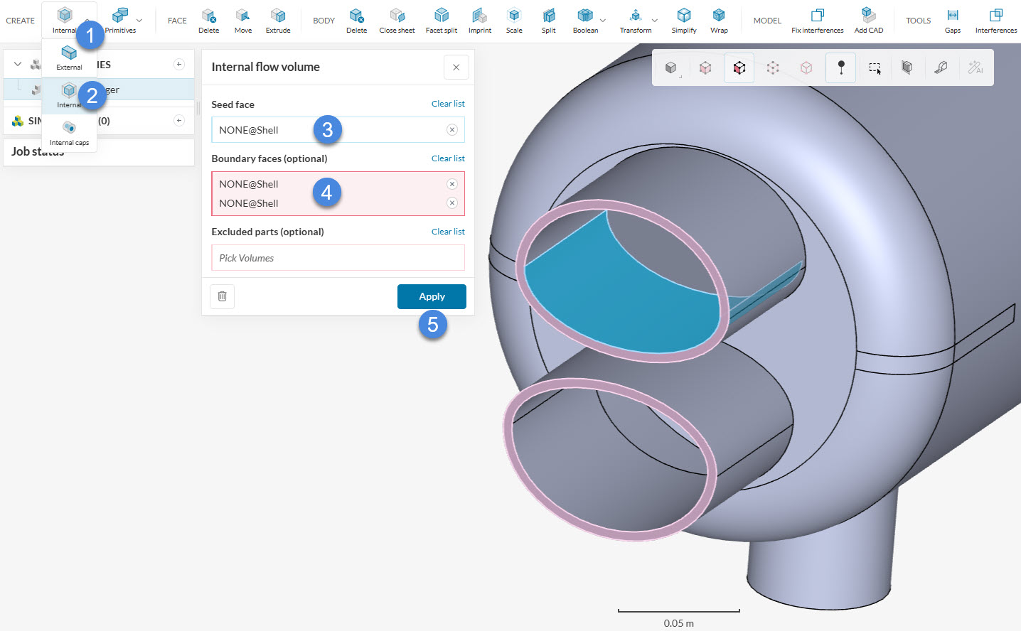
1. Create an ‘Internal Flow Volume’ operation;
2. Define a Seed face, which is a face that will be in contact with the flow region. In Figure 5, the seed face is highlighted in blue;
3. Select the Boundary faces, where the openings are. In this case, you have two boundary faces, highlighted in white in Figure 5;
4. Hit ‘Apply’.

At this point, the tube side flow region will be created. Using the same logic, you have to create one more flow region, using another internal flow volume operation:

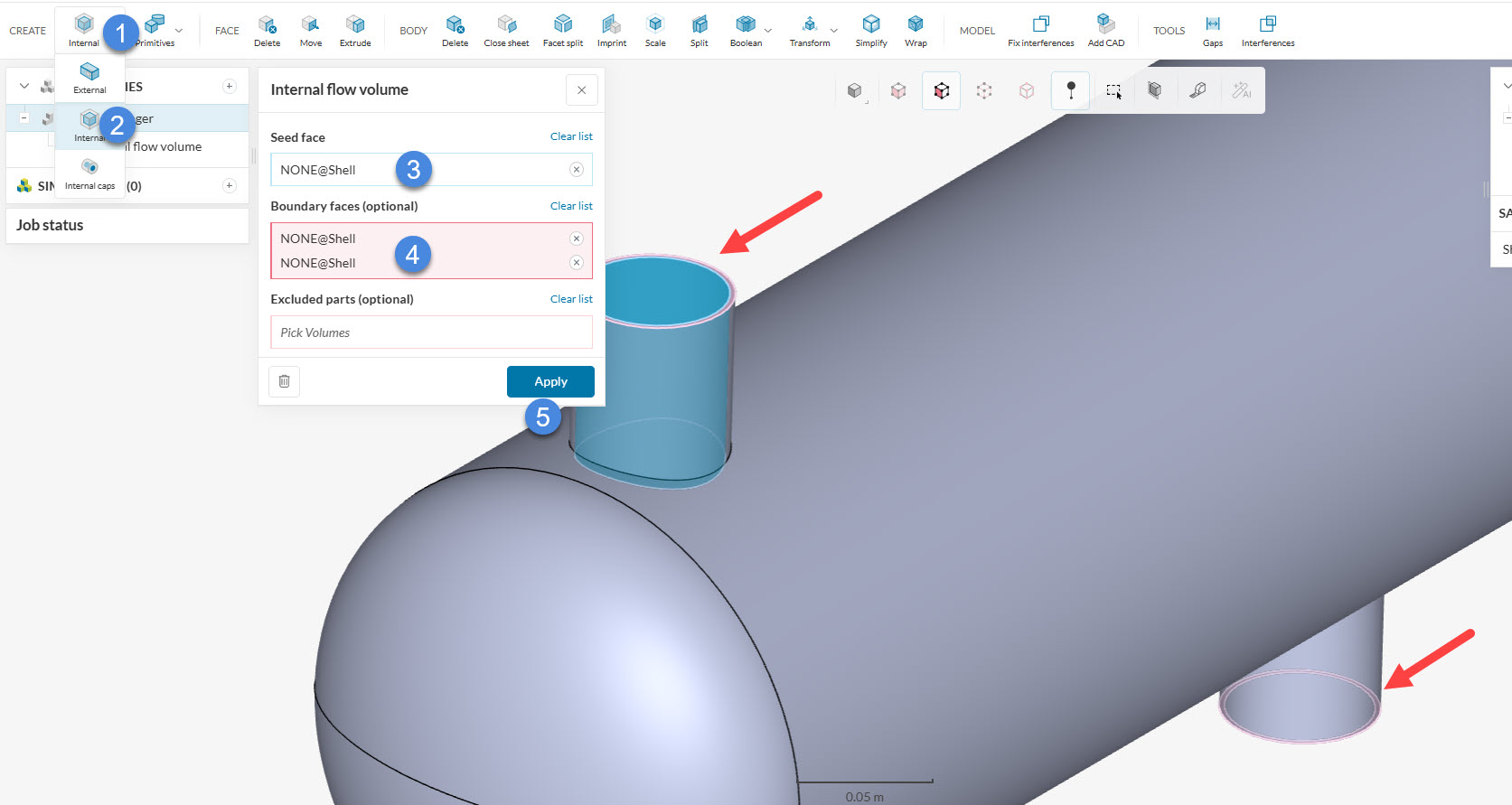
In the image above, please note that you will need to rotate the model around to select the second boundary face.

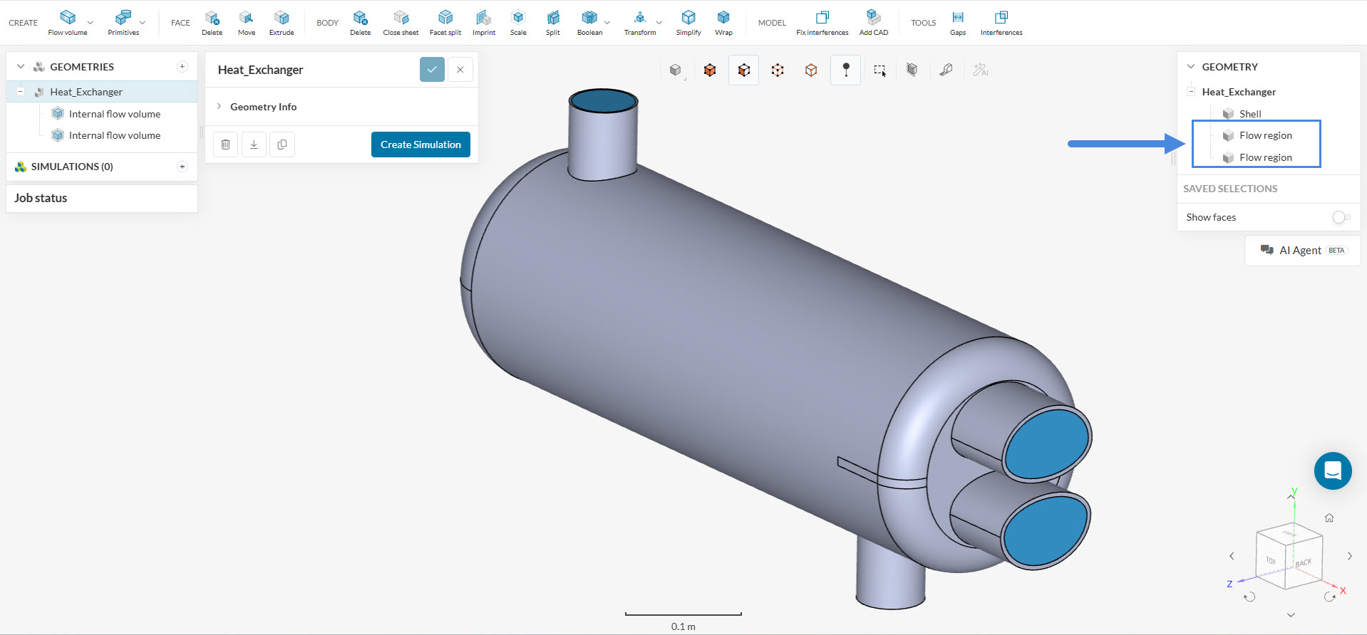
Now you have both fluid regions ready for the u-tube heat exchanger. Only the Imprint operation is missing before the model is ready to simulate:

1. Select an ‘Imprint’ operation
2. Click ‘Apply’
3. Hit ‘Save as copy’ to add the finalized model to your Workbench

1.3. Create the U-tube Heat Exchanger Simulation

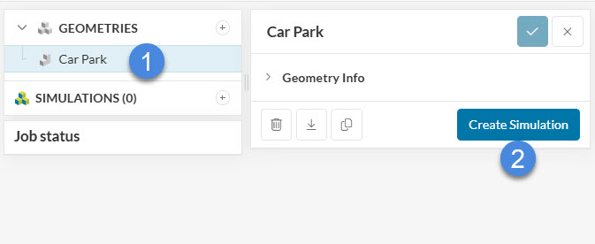
When a model the exported from CAD Mode, it will be named Copy of Heat_Exchanger. This is the model that we will use to run the simulation. Before ‘Creating a Simulation’, you can also rename the CAD model appropriately, and save the changes by clicking on the check icon.

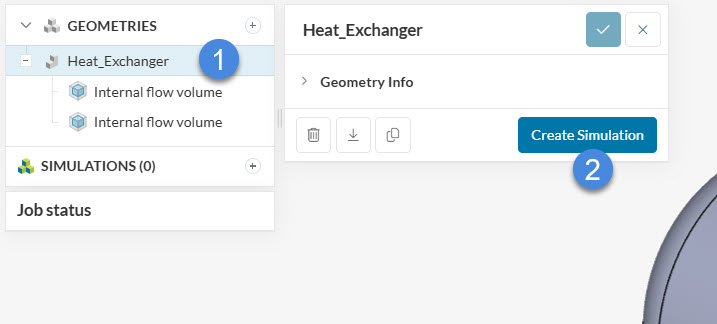
At this point, the analysis type widget opens in the viewer:

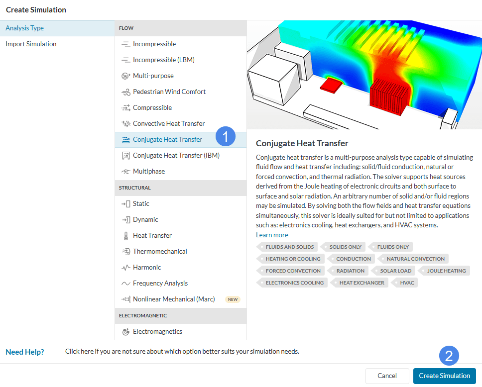
Choose the ‘Conjugate Heat Transfer v2.0’, then click on the ‘Create Simulation’ button to get started. If you want to learn more about this analysis type, click here.

2. Setting Up the U-tube Heat Exchanger Simulation

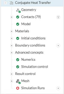
Now you can define the global settings of your u-tube heat exchanger simulation. The following setup should pop up automatically, if not you get there by clicking on the name of the simulation:

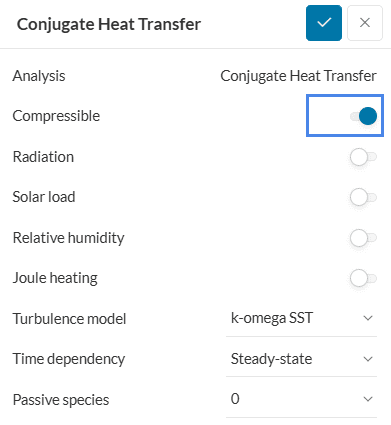
Here, you can define global settings for your simulation. In this case, the flow is turbulent, so the ‘k-omega SST’ turbulence model is chosen and the ‘Compressible’ option is enabled to account for the density variations within the domain.

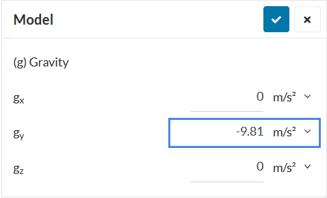
2.1. Assign the Model

Click on ‘Model’ in the simulation tree to define the gravity force acting on the domain according to the coordinate system of the CAD. In this case, gravity is defined in the negative y-direction:

2.2. Assign the Materials

In this simulation, you want to analyze the heat transfer between a fluid through a solid into another fluid. Therefore, you need to assign properties to the two-fluid regions and the solid shell.

a. Fluids

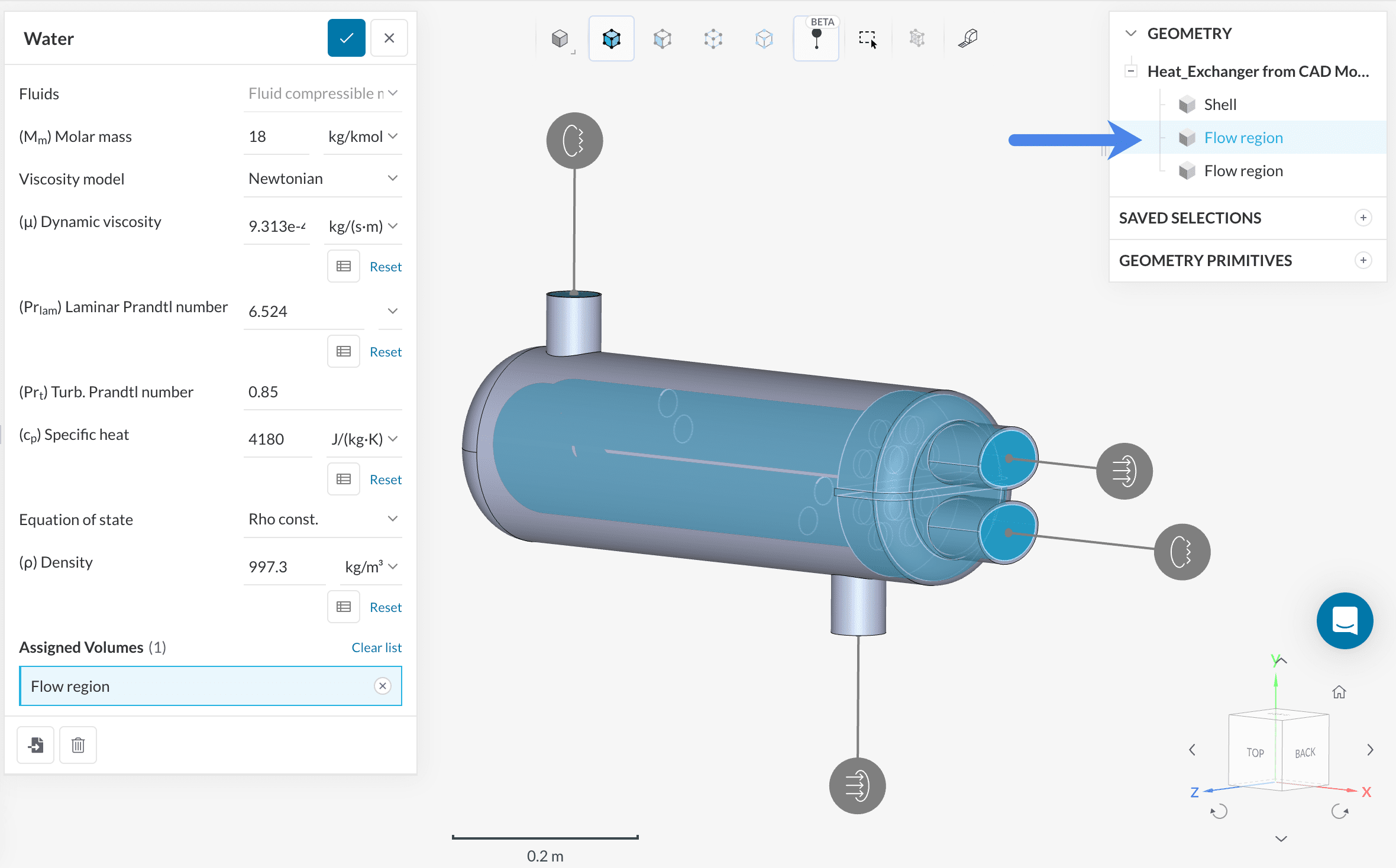
To apply a new material, click on the ‘+’ icon next to the Fluids under the Materials tab. For this project, the two flow regions consist of ‘Water’, so choose it from the option that is listed on the panel that appears:

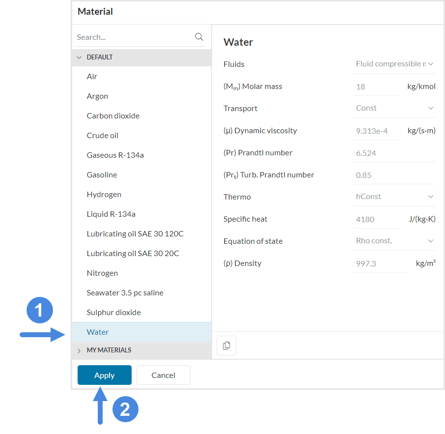
After you click ‘Apply’, assign the material to the inner flow region by picking it on the geometry tree at the top right of the screen.

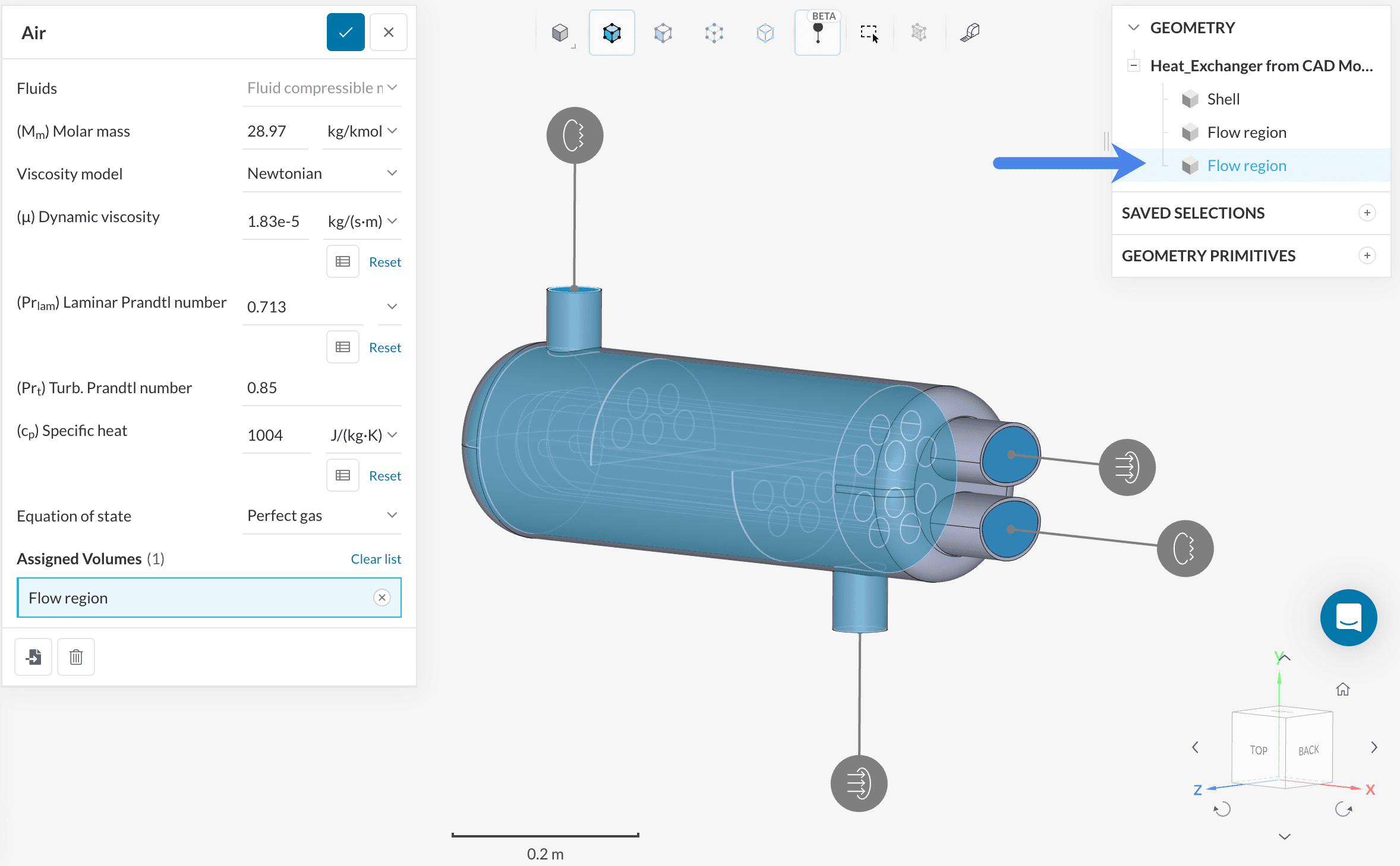
Now you will assign ‘Air’ as material of the hot flow region:

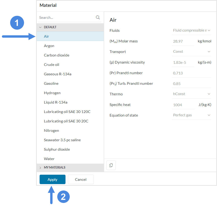
Pick the flow region that corresponds to the outer fluid part:

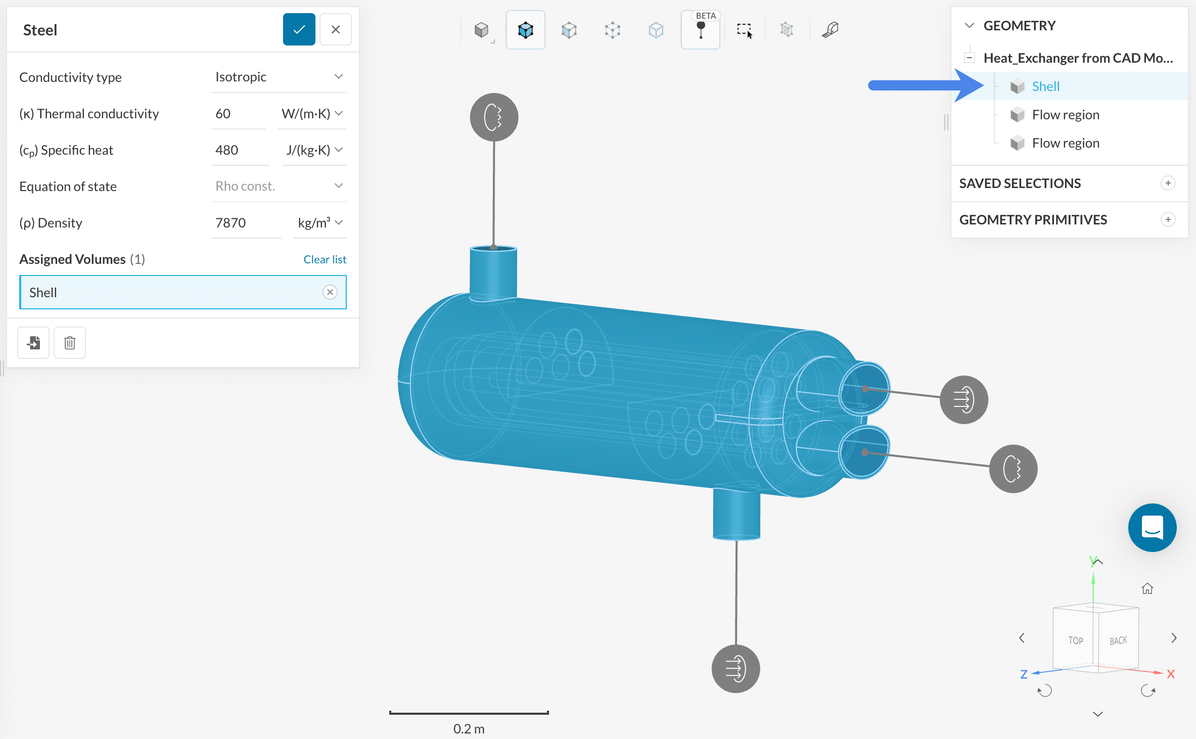
Solids

Click on the ‘+’ icon next to the Solids under the Materials tab. The material chosen for the shell is ‘Steel’.

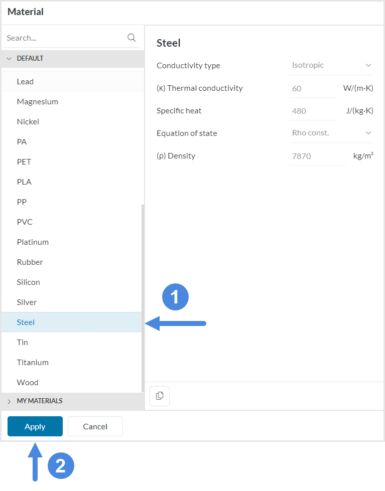
The same procedure is followed to assign it to the respective part:

2.3. Assign the Boundary Conditions

To assign boundary conditions on the u-tube heat exchanger, click on the ‘+‘ icon next to the Boundary conditions, and click on the types described in this section.

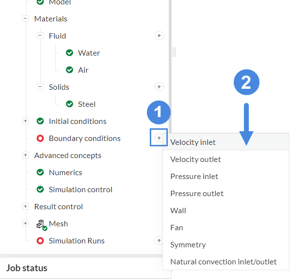
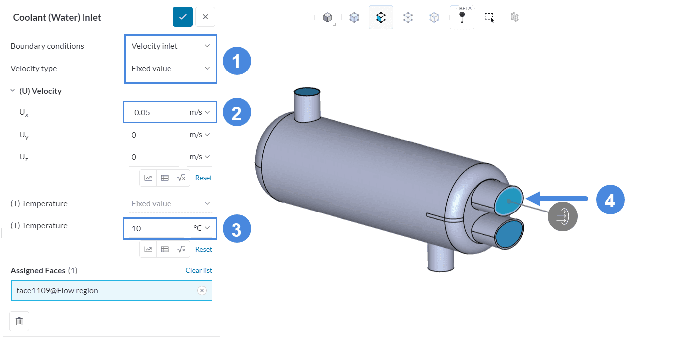
Inner Flow Region (Low-Temperature Fluid Region)

Initially, apply the inlet velocity of the cold stream, by clicking on the ‘Velocity Inlet’ option from the drop-down menu that appears as seen in Figure 18, and set the velocity in the x-direction to ‘-0.05’ \(m \over s \). Add a temperature of ’10’ \(°C\).

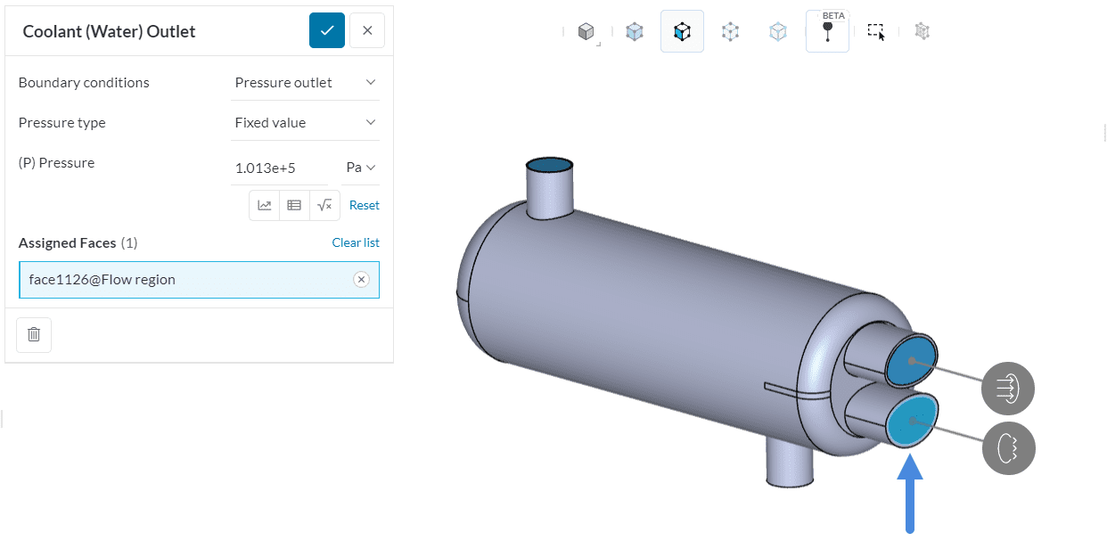
A Pressure Outlet condition with a fixed value of the atmospheric pressure ‘101325’ \(Pa\) is then applied to the outlet face of the inner flow region:

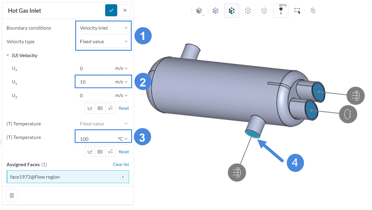
Outer Flow Region (High-Temperature Fluid Region)

Apply the same procedure for the hot stream, aka the outer flow region as well, starting with a Velocity of ’10’ \( m \over s\) in the y-direction and a temperature of ‘100’ \(°C\).

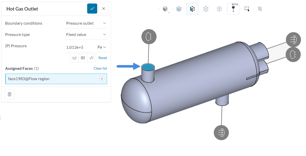
Finally, set the Pressure Outlet condition for the outlet with a fixed value of ‘101325’ \(Pa\):

2.5. Simulation Control & Numerics

Leave the Simulation Control and Numerics panel at its default state, since the default settings are optimized enough for this application.

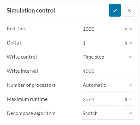
These simulation control settings will perform 1000 iterations and only print one solution field at the latest iteration. If you want to know more about simulation control settings, you can check out this page for more information.

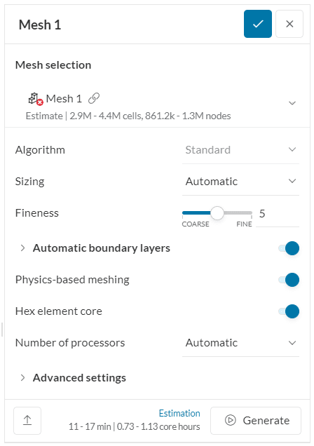
3. Mesh

Click on ‘Mesh’ to access the global mesh settings, shown in the following picture. Choose the ‘Standard’ algorithm, and set the Fineness to Level ‘5’:

If you are interested to see how to use the standard meshing tool, take a look at this tutorial.

4. Start the U-tube Heat Exchanger Simulation

After all the settings are completed, proceed by clicking the ‘+’ icon next to the Simulation Runs, so you start with the analysis. The mesh will be generated automatically before the run.

While the results are being calculated, you can already have a look at the intermediate results in the post-processor. They are being updated in real-time!

5. Post-Processing

When the simulation is complete, you can check the Convergence and the Results of the simulation. You can access either of them in the Simulation tree by clicking on them, as you can see below:

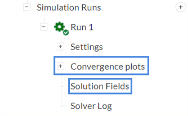
5.1. Convergence Plot

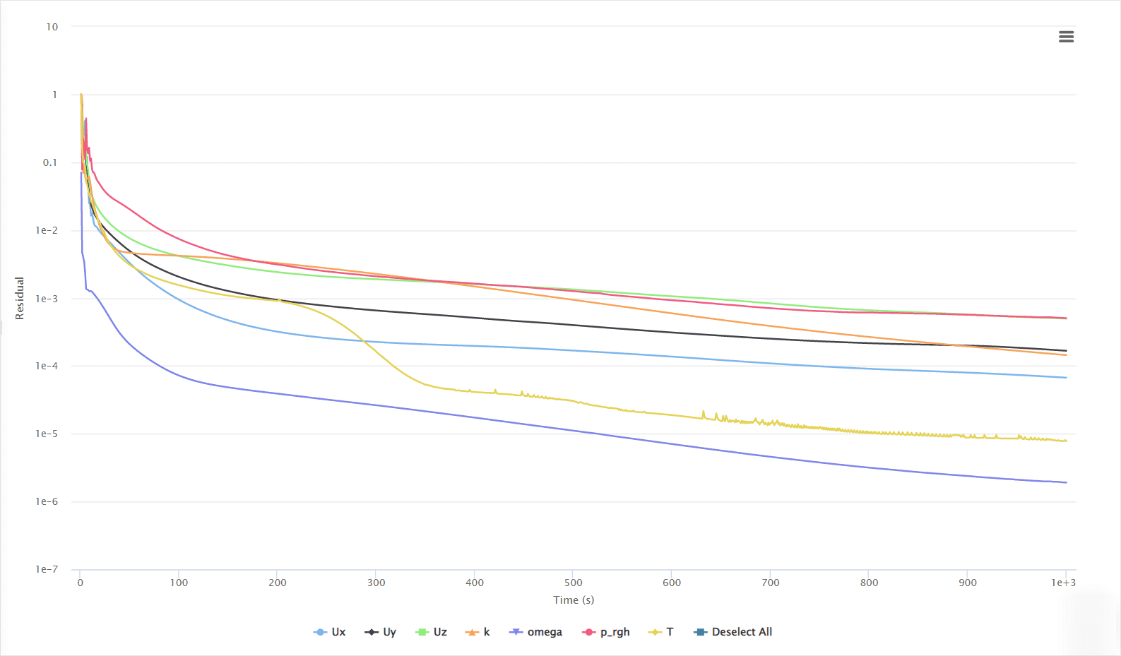
The convergence plot indicates whether or not the solution is reliable, or whether some changes should be made in the settings, such as making the mesh finer or increasing the simulation time. In the following picture, you can see how the residuals of your simulations will appear in the plot:

To view the results of your u-tube heat exchanger simulation, click on the ‘Solution Fields’ tab under your finished run. This will redirect you to the post-processor.

5.2 Surface Visualization of U-tube Heat Exchanger

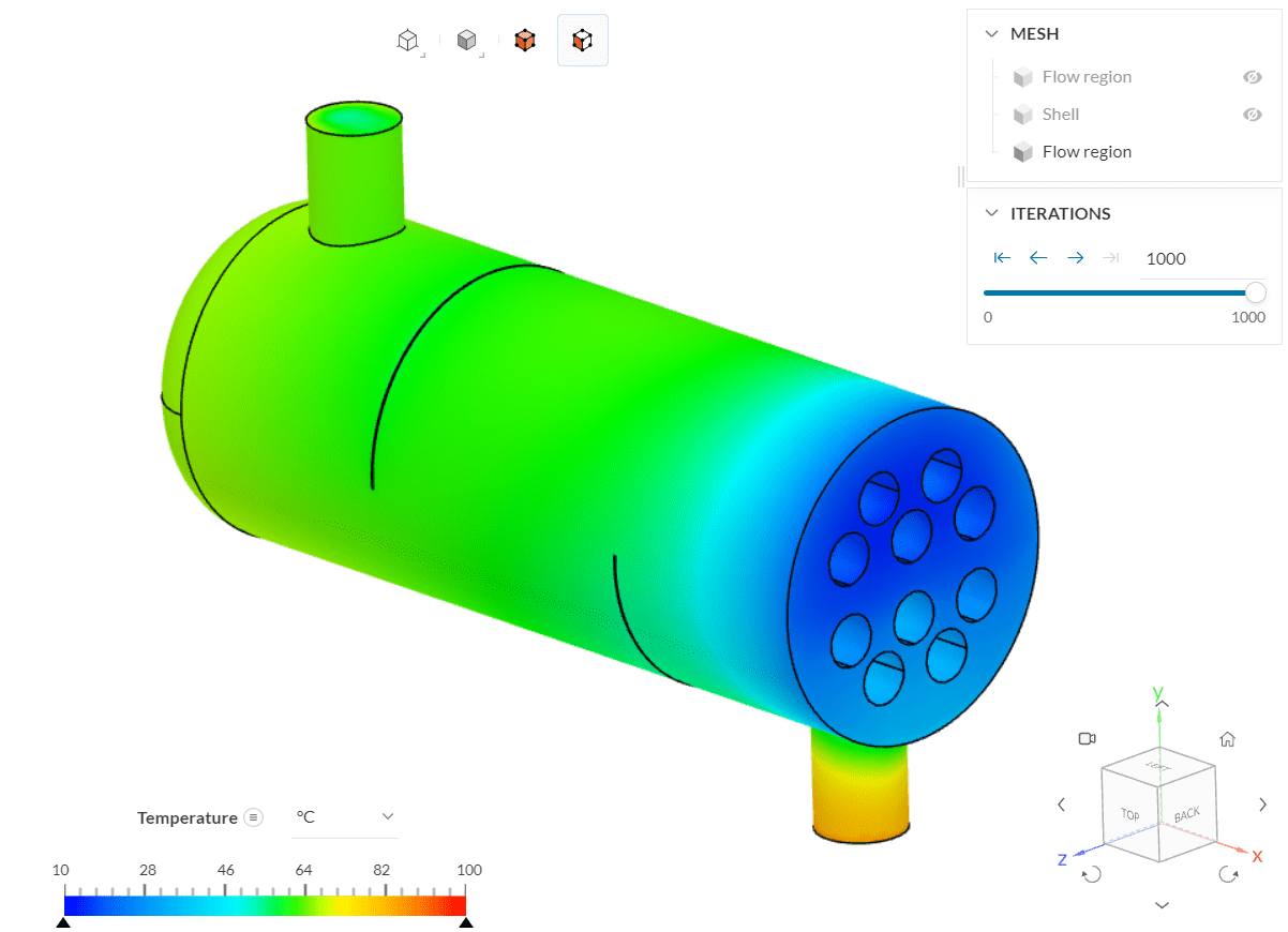
You can check the distribution of a parameter across a whole part. For example. if you wish to view the temperature values of the hot gas, do the following:

• Hide the flow region that corresponds to the coolant, as well as the shell using the tree at the top right;
• Set the Coloring input to ‘Temperature’;
• Change the unit to ‘\(°C\)’;
• Right-click on the legend at the bottom and choose the ‘Use continuous legend’ option.

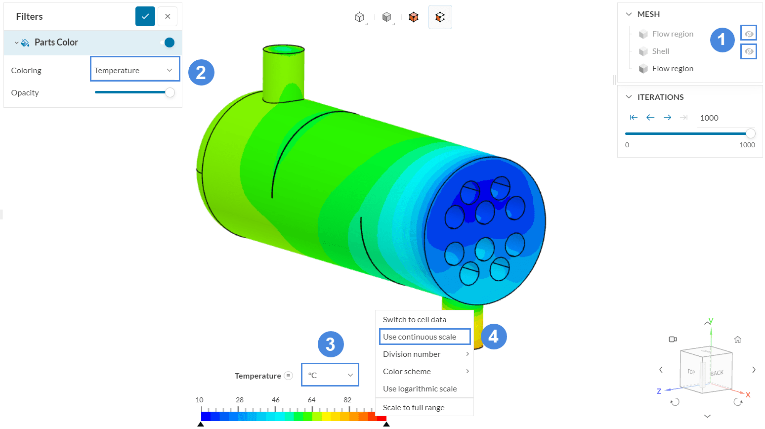
The drop of the high-temperature inlet to the low-temperature outlet can be seen due to the transition of warm colors at the bottom to cold shades at the upper side of the fluid domain.

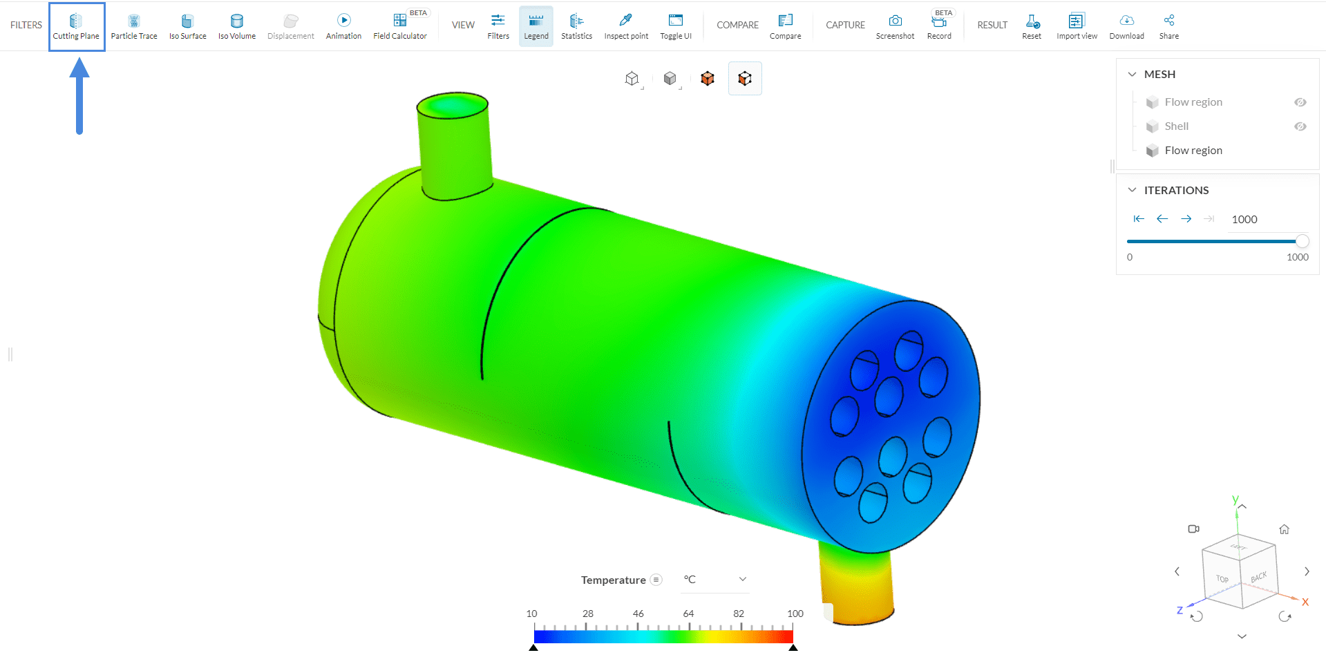
5.2. Cutting Planes

Create a new cutting plane to view the temperature distribution across the center plane. To add this feature:

• Click on the ‘Cutting Plane’ option;

• Choose the ‘Z’ axis. It will automatically generate a plane normal to this axis, coincident with the origin of the model. If you wish to visualize the plane as in Figure 31, make sure you check the inversion button next to the orientation option;
• Choose ‘Temperature’ as the Coloring option.

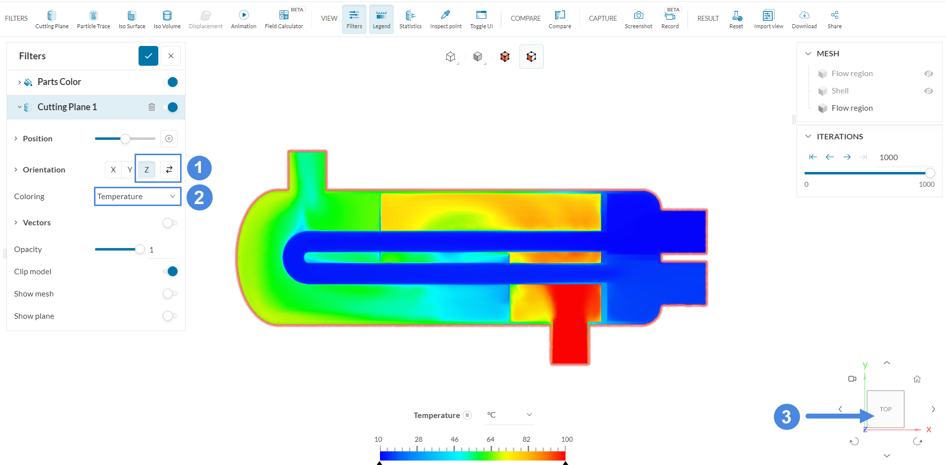
Now the contribution of the coolant in the temperature drop of the hot gas can also be visualized. The areas that are close to the hot gas inlet appear warmer than the upper part which is located near the cooler side. Also, the left part of the cutting plane, which is the farthest away from the coolant, has some warm-colored contours as well.

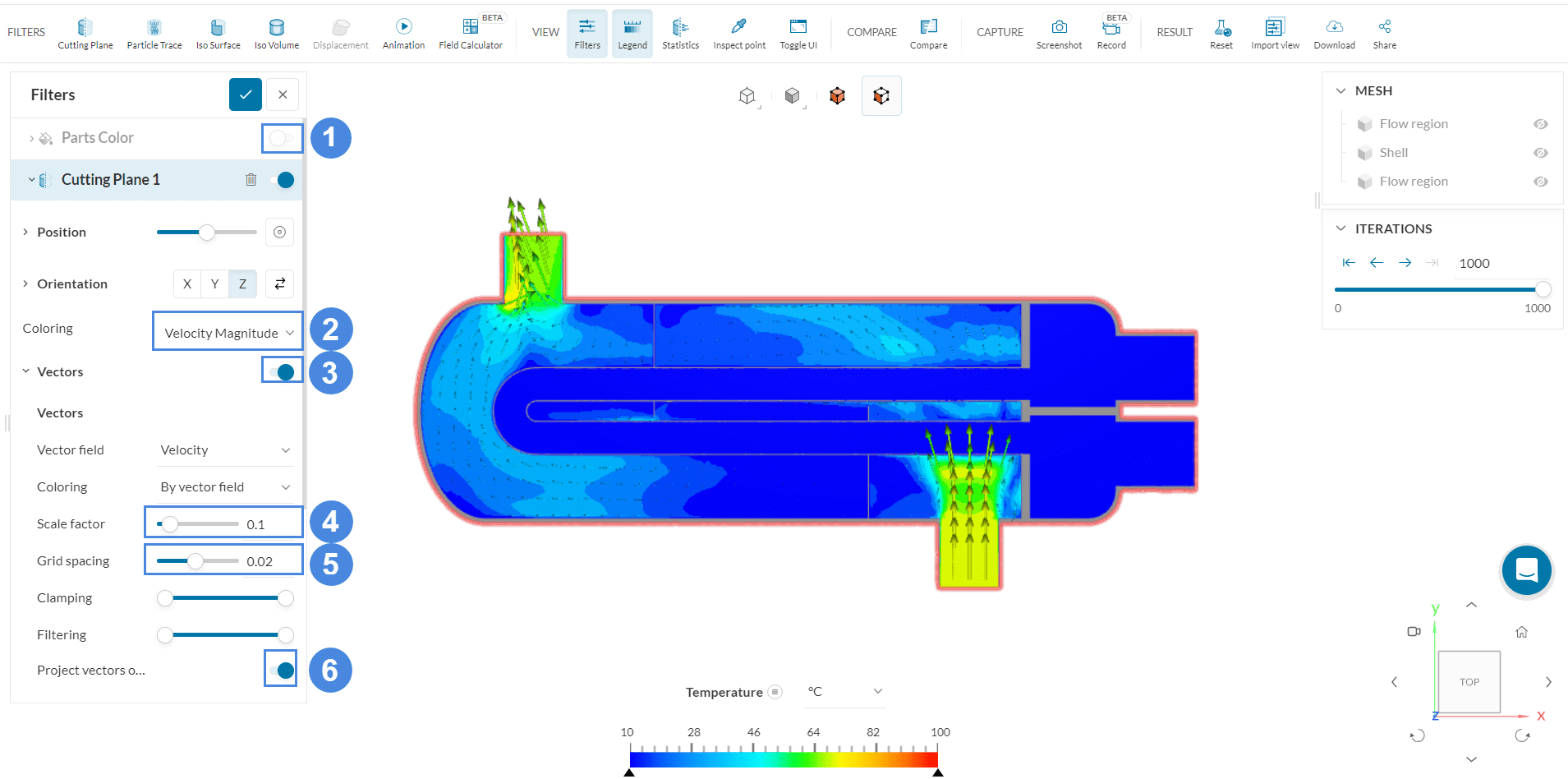
Apart from the internal temperature, the velocity magnitude can be really insightful too, especially when the vectors are visualized:

• Deactivate the Parts Color, so only the plane is displayed on the screen;
• Change the Coloring to ‘Velocity Magnitude’;
• Activate the ‘Vectors’;
• Change the Scale factor to ‘0.1’ and the Grid Spacing to ‘0.02’;
• Finally, activate the ‘Project vectors onto plane’.

5.3. Streamlines

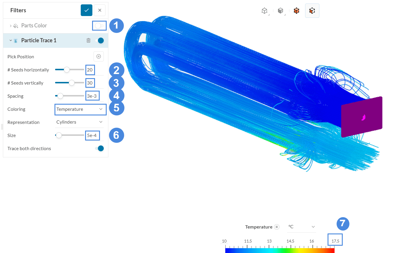
Create a Particle Trace set, and select the face of the inlet’s coolant as the seed face in order to generate the visualization of flow as streamlines:

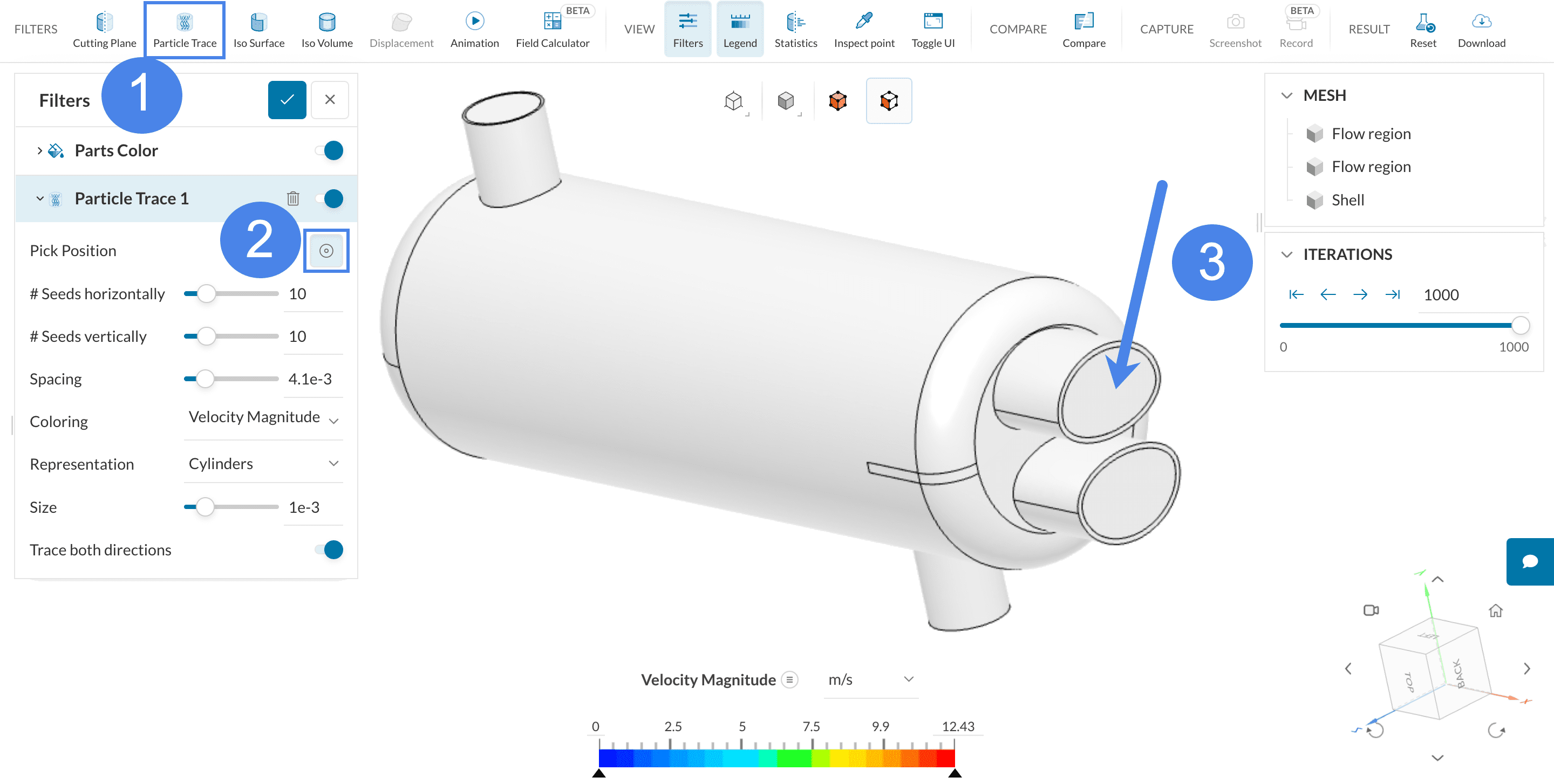
• Deactivate the visualization of Parts Color, so you only see the streamlines on the workbench;
• Set the number of streamlines that are going to be generated horizontally to ’20’. Repeat for the number of streamlines that are going to be generated vertically, but this time set it to ’30’;
• Add a Spacing input of ‘3e-3’;
• Switch the Coloring to ‘Temperature’;
• Set the Size to ‘5e-4’. This is the diameter of the streamlines’ circular cross-section;
• For this case, the Trace both directions option can be both activated or deactivated.

This can be repeated for the hot gas too. Create a new ‘Particle Trace’ set. Select the face of the inlet as the seed face too:

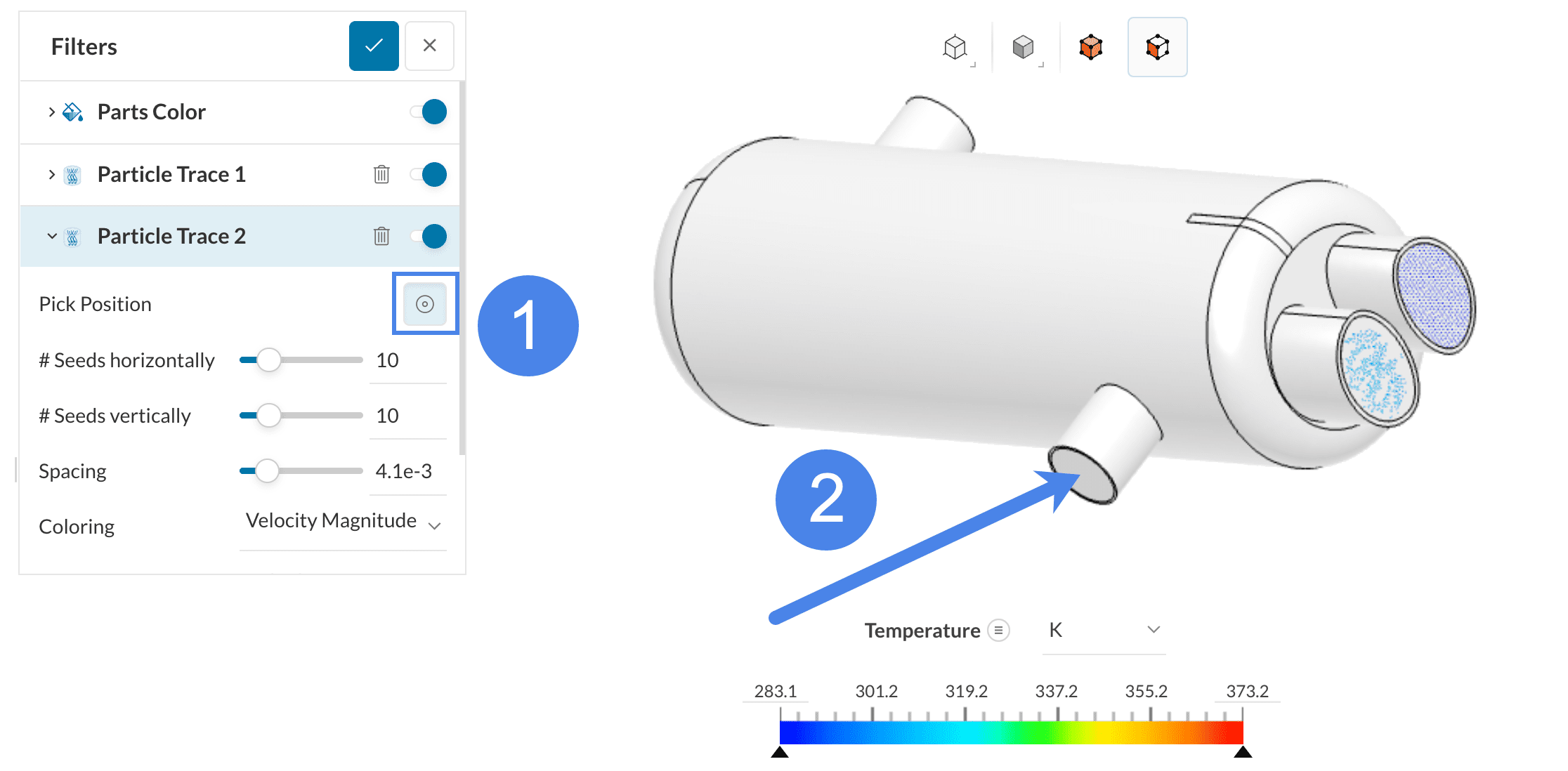
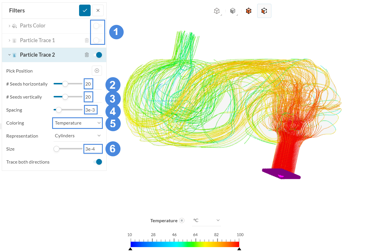
Then apply the following:

• Deactivate the two filters from before so you only see the new set of streamlines;
• Set the # Seeds horizontally and # Seeds vertically to ’20’;
• Add a Spacing input of ‘3e-3’;
• Switch the Coloring to ‘Temperature’;
• Set the Size to ‘3e-4’;
• Deactivate the Trace both directions option.

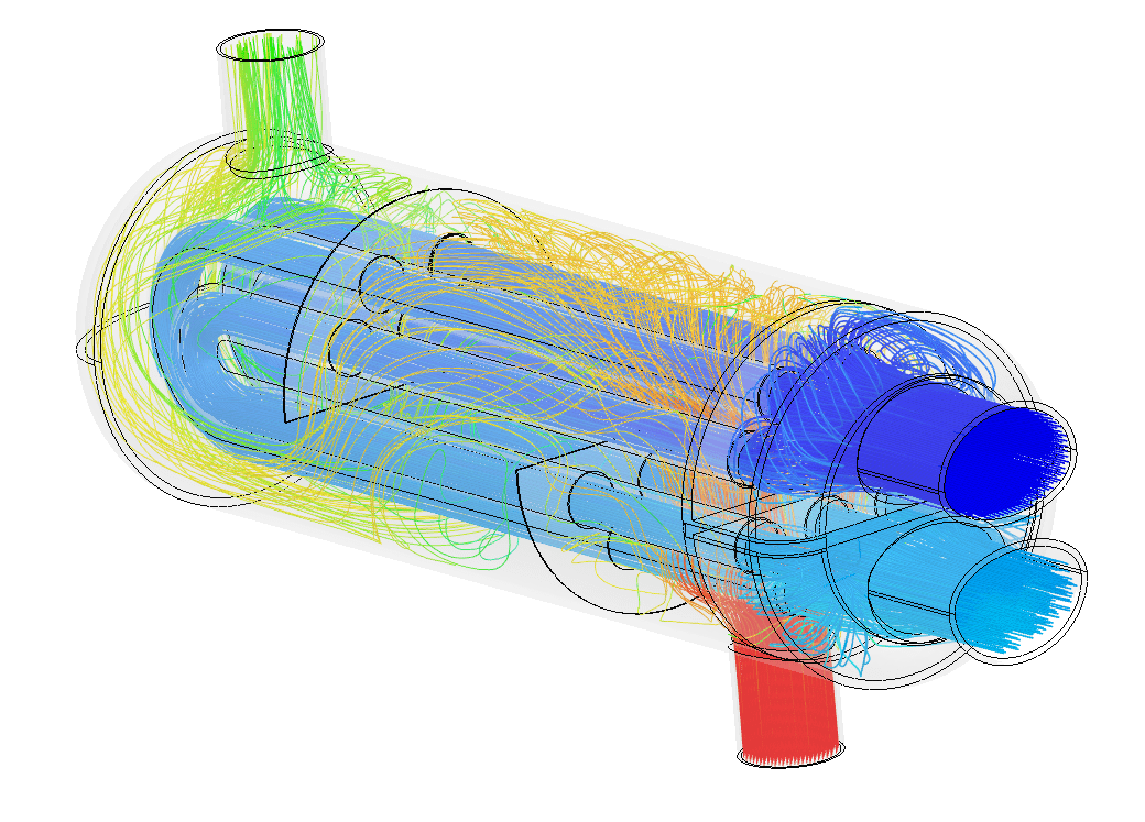
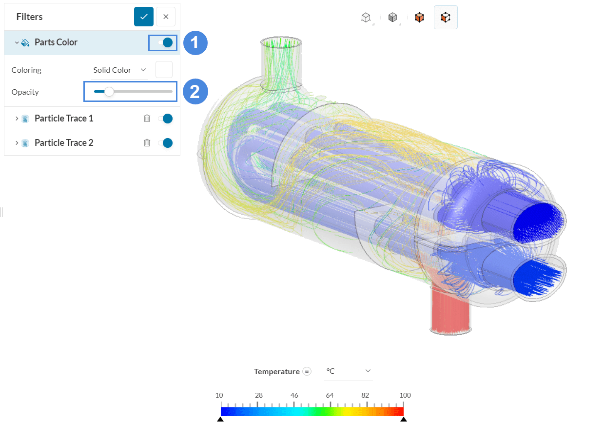
Finally, keep in mind that if you wish to visualize the streamlines and the shell at the same time, so you produce an image as you can see in Figure 1, then you can go ahead and reduce the opacity of the latter, after setting the Coloring to ‘Solid Color’:

For more information, have a look at our post-processing guide to learn how to use the post-processor.
Congratulations! You finished the tutorial!

Last updated: November 21st, 2023

What's Next

Thermal Management of an Electronics Box using CHT Analysis