Documentation
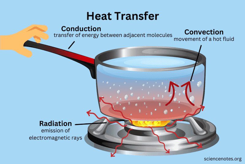
Conduction is one of the three main ways that thermal energy is transferred from one place to another: conduction, convection (quantified by the Nusselt number), and radiation. It is caused by collisions between neighbouring atoms or molecules, predominantly in a solid or liquid substance. Conduction is more significant in materials where particles are closely packed together as opposed to the ones where they are further apart.
The rate of conduction is higher when there is a large temperature difference between the substances that are in contact with each other. A classic example of conduction is when you notice the handle of a pan with hot water gets warm after a few minutes. Anything that involves direct physical contact to transfer heat is an example of conduction.
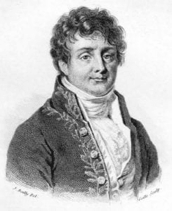
The transient process of heat conduction, described by a partial differential equation, was first formulated by Jean Baptiste Joseph Fourier (1768-1830) and was presented as a manuscript to the Institut de France in 1807. However, fifteen years after publishing his manuscript, Fourier formulated a complete theory on heat conduction in his book “Théorie Analytique de la Chaleur” in 1822.
Fourier’s law states that heat flux is directly proportional to the magnitude of the temperature gradient.
$$q=-k\frac{\Delta T}{\Delta x}$$
where,
k = proportionality constant, quantifies the thermal conductivity of the material
\(\frac{\Delta T}{\Delta x}\) = temperature gradient, change in temperature \(\left(\Delta T\right)\) as a function of position \(\left(\Delta x\right)\)
Note: Heat flux is a vector quantity, where a decrease in temperature with x leads to a positive value of q flowing in the positive x direction and vice versa. In other words, heat flows from the hot to the cold temperature. The equivalent three-dimensional form is:
$$\bar q=-k \nabla T$$
where, \(\nabla\) indicates the gradient.
The rate of heat flow is the amount of heat that is transferred per unit of time in some material, usually measured in Watt (joules per second). Based on Fourier’s Law of Heat Conduction, the rate of heat flow is:
$$\frac{Q}{\Delta t}=-kA\frac{\Delta T}{\Delta x}$$
where,
Q = net heat transfer in W
\(\Delta t\) = time taken in s
\(\Delta T\) = time difference in temperature between the cold and hot sides in K
\(\Delta x\) = thickness of the material conducting heat (distance between hot and cold sides) in m
k = thermal conductivity in W/(m.K)
A = surface area of the surface-emitting heat in m2
When we think of a conduction problem, the following few parameters contribute to the rate at which heat transfer occurs:
Conduction depends on geometrical properties like the cross-sectional area A and the thickness of a material \(\Delta x\).
$$\dot Q \propto A$$
$$\dot Q \propto \frac{1}{\Delta x}$$
The larger the area, the faster the heat transfer will happen since more collisions occur between the molecules. In contrast, the thickness of the material is inversely proportional to the heat transfer rate.
Conduction occurs only when there is a temperature difference either within different sections of a material or between two materials in contact. Furthermore, the higher the temperature difference, the higher the heat transfer per unit of time.
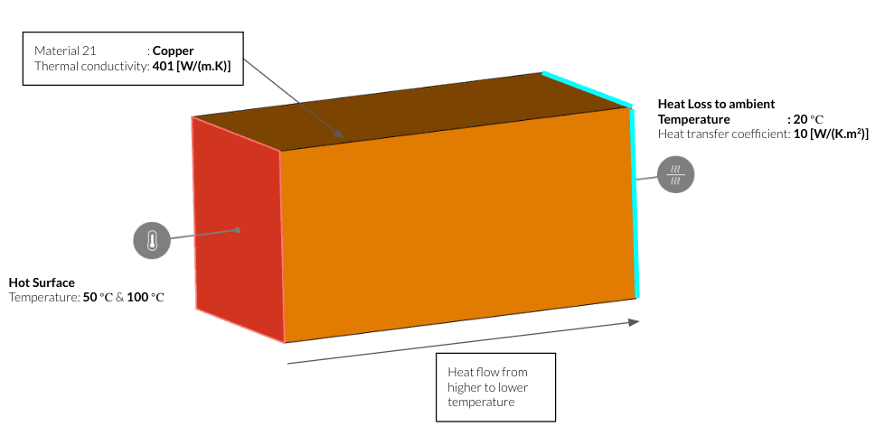
To understand this behaviour, we can simulate two different temperature gradients easily using SimScale’s Heat Transfer analysis. Let’s consider a solid material with a hot and cold side.
| Case | Hot Side | Cold Side |
| 1 | 50° C | 20° C with a heat loss of 10 W/K.m2 |
| 2 | 100° C | 20° C with a heat loss of 10 W/K.m2 |
Once the simulations are finished, with the compare filter in SimScale you can clearly see a qualitative difference between the cases below:
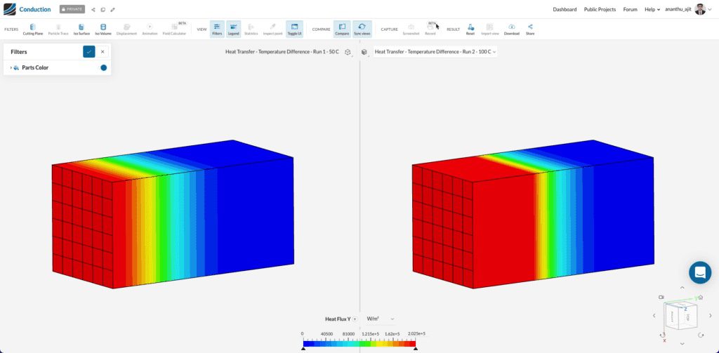
With the exact material properties and 10 seconds of transient simulation, the heat flux through the second case is much higher than the first due to a greater temperature difference. This can be seen quantitatively using the heat flow result monitor on the hot surface.
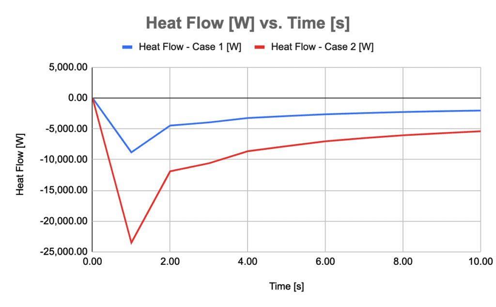
In comparison, with 10 seconds of run time, the case with a higher temperature difference (100° C) shows a higher heat flow.
Note: The negative values of heat flow represent the heat loss from the hot surface according to Fourier’s Law of Heat Conduction.
Thermal conductivity of a material quantifies the ability to conduct heat. Each material has its own thermal conductivity based on the arrangement of electrons in them. Some materials, e.g. metals, conduct heat easily.
In principle, the presence of free electrons in them makes the collisions between molecules faster, leading to better conductivity. Materials behave as thermal conductors when they have higher thermal conductivity and as insulators with lower thermal conductivity.
For gasses the interaction of molecules determines their thermal conductivity. Molecules inside a material move from one position to another as shown in the picture below:
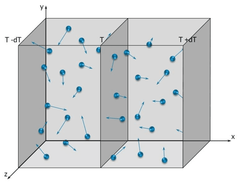
The internal energy of the molecules is transferred by impact with other molecules. As a result, areas with low temperatures will be occupied by molecules of high temperatures and vice-versa. The thermal conductivity can be explained with this model and be derived from the kinetic theory of gasses [4]:
$$T=\frac{2}{3} \frac{K}{N\left(k_B\right)}$$
where,
K = kinetic energy of the molecules
N = number of moles
kB = Boltzmann constant
T = absolute temperature
which states that “the average molecular kinetic energy is directly proportional to the absolute temperature for an ideal gas” [6]. It is important to note that, the thermal conductivity is independent of the pressure and increases with the root of the temperature.
In general, the kinetic theory is pretty hard to understand for objects other than gasses. And for fluids, it is even more difficult because there is no simple theory. In nonmetallic components, heat transfer happens via lattice vibrations (Phonon), which is beyond the scope of this article.
The table below shows the thermal conductivity of some common materials [5]:
| Material | Thermal Conductivity K \(\frac{W}{\text {m.K}}\) |
| Silver | 429 |
| Copper | 401 |
| Aluminum | 235 |
| Steel | 60 |
| Cast Iron | 52 |
| Concrete | 0.8 |
| Glass | 0.6 |
| Wood | 0.16 |
| Air | 0.023 |
An example heat transfer analysis shows how the heat flows within materials with three different thermal conductivities. The case is set up with a fixed temperature on the top and a convective heat loss on the bottom.
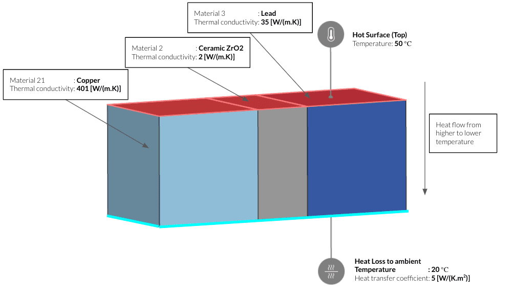
Running the simulation for 50 seconds shows variations in the heat flow according to the thermal conductivity of the materials. The block on the left made of copper shows a faster heat flow in comparison to the other two with lower thermal conductivity. Whereas the central block made of ceramic almost acts as an insulator between copper and lead due to its extremely low thermal conductivity \(2 \frac{W}{\text {m.K}}\).
Note: In building thermal performance, thermal conductivity and material thickness are combined to define the R and U value of the insulation materials. To find out more about how thermal insulations affect the comfort and performance of building fabric, please take a look at our webinar on “Fabric First: CFD for Passive Environmental Design”.
Temperature scalar value for each node in the model.
Heat flux vector for each node in the model, expressed in global components X, Y, Z. It has units of energy per unit of time per unit of area \(\frac{J}{\left(s\right)m^2}\) or units of power per unit of area \(\frac{W}{m^2}\).
Available as an area calculation, retrieves the total heat per unit time \(\frac{𝐽}{𝑠}\), or power (𝑊), leaving or entering the domain through the selected faces. This field is computed as the integral of the Heat Flux over the selected surface.
In thermodynamics, the heat transfer coefficient or film coefficient, or film effectiveness, is the proportionality constant between the heat flux and the temperature difference [3]. It is generally calculated on the surface of a material as it is caused by the temperature difference between the boundary of a material and the external environment. The unit of heat transfer coefficient is \(\frac{W}{\text{K.m}^2}\).
The general definition of the heat transfer coefficient is:
$$h=\frac{q}{\Delta T}$$
where,
h = heat transfer coefficient
q = heat flux in \(\frac{W}{m^2}\)
\(\Delta T\) = difference in temperature between the surface of the material and the surrounding fluid/environment
In a pure conduction-based simulation, the heat transfer coefficient is supplied as an input for the heat loss from the boundary of the material used. On the other hand, to determine the heat transfer coefficient of a material with defined flow conditions, the Conjugate Heat Transfer v2 analysis should be performed.
To know how to enable the heat transfer coefficient output within SimScale, refer to the article on field calculations.
Designers and engineers can solve a conduction-based case using SimScale’s heat transfer analysis under the structural module. With SimScale’s easy-to-set-up workflow, you will be able to import your 3D CAD model, apply the physical and thermal constraints, and start the simulation within minutes. The tutorial on Thermal Analysis of a Differential Casing should provide detailed setup information to get an overview of a heat transfer simulation workflow within SimScale.

To get started with SimScale, users can easily sign up here. With the cloud-native approach, users can start any number of parallel simulations using just a personal laptop and an internet connection.
References
Last updated: March 16th, 2026
We appreciate and value your feedback.
What's Next
What is Convection?Sign up for SimScale
and start simulating now


