What Are Boundary Conditions?
Boundary conditions are constraints necessary for the solution of a boundary value problem. A boundary value problem is a differential equation (or system of differential equations) to be solved in a domain on whose boundary a set of conditions is known. It is opposed to the “initial value problem”, in which only the conditions on one extreme of the interval are known.
Boundary value problems are extremely important as they model a vast amount of phenomena and applications, from solid mechanics to heat transfer, fluid mechanics, and acoustic diffusion. They arise naturally in every problem based on a differential equation to be solved in space, while initial value problems usually refer to problems to be solved in time.
Boundary value problems have been extensively studied by Jacques Charles François Sturm (1803-1855) and Joseph Liouville (1809-1882), who studied the eigenvalues of a linear differential equation of the second order\(^1\). They studied the conditions that guarantee the existence and uniqueness of the solution of the differential problem and how it is affected by the boundary conditions\(^2\). The Sturm-Liouville theory is extremely important for any computational problem because it enables us to understand if a problem is “well-posed” and how it is possible to obtain the solution.
Types of Boundary Conditions
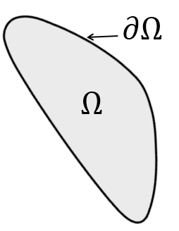
Both ordinary and partial differential equations require solving boundary conditions (B.C.). Different types of boundary conditions can be imposed on the boundary of the domain (Figure 1). The choice of the boundary condition is fundamental for the resolution of the computational problem: a bad imposition of B.C. may lead to the divergence of the solution or to the convergence of a wrong solution.
There are five types of boundary conditions:
- Dirichlet boundary condition (also known as Type I)
- Neumann boundary condition (also known as Type II)
- Robin boundary condition (also known as Type III)
- Mixed boundary condition
- Cauchy boundary condition
Dirichlet Boundary Condition
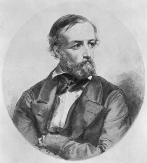
The Dirichlet boundary condition is a type of boundary condition named after Peter Gustav Lejeune Dirichlet (1805–1859, Figure 2)\(^3\).
This condition specifies the value that the unknown function needs to take on along the boundary of the domain. Given, for example, the Laplace equation, the boundary value problem with the Dirichlet b.c. is written as:
$$ \Delta \varphi (\underline{x}) = 0 \qquad \forall \underline{x}\in \Omega \tag{1}$$
$$ \varphi (\underline{x}) = f(\underline{x}) \qquad \forall \underline{x}\in \partial \Omega \tag{2}$$
where \(\varphi\) is the unknown function, \(\underline{x}\) is the independent variable (e.g. the spatial coordinates), \(\Omega\) is the function domain, \(\partial\Omega\) is the boundary of the domain, and \(f\) is a given scalar function defined on \(\partial\Omega\). In the framework of numerical simulations, it is usually imposed directly in the algebraic system to be solved. Let’s consider the following algebraic system derived from a numerical algorithm:
$$ \begin{bmatrix}
k_{1,1} & k_{1,2} & . & k_{1,m-1} & k_{1,m}\\ k_{2,1} & k_{2,2} & . & k_{2,m-1} & k_{2,m}\\ . & . & . & . & . \\ k_{m-1,1} & k_{m-1,2} & . & k_{m-1,m-1} & k_{m-1,m}\\ k_{m,1} & k_{m,2} & . & k_{m,m-1} & k_{m,m} \end{bmatrix} \begin{bmatrix} x_1\\ x_2\\ .\\ x_{n-1}\\ x_n \end{bmatrix} = \begin{bmatrix} a_1\\ a_2\\ .\\ a_{m-1}\\ a_m \end{bmatrix} $$
where \(k_{ij}\) are the elements of the algebraic operator (e.g. the stiffness matrix), \(x_i\) are the unknowns (i.e. the degrees of freedom of the problem), and \(a_i\) are the known terms. The simplest way to impose a Dirichlet boundary condition on the \(n^{th}\) degree of freedom is to modify the system as follows:
$$ \begin{bmatrix}
k_{1,1} & . & . & . & k_{1,m}\\ . & . & . & . & .\\ 0 & 0 & 1 & 0 & 0 \\ . & . & . & . & . \\ k_{m,1} & . & . & . & k_{m,m} \end{bmatrix} \begin{bmatrix} x_1\\ .\\ x_n\\ .\\ x_m \end{bmatrix} = \begin{bmatrix} a_1\\ .\\ f\\ .\\ a_m \end{bmatrix} $$
where \(f\) is the value that the \(n^{th}\) degree of freedom must be taking.
Neumann Boundary Condition
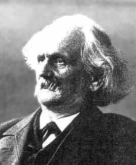
The Neumann boundary condition is a type of boundary condition named after Carl Neumann (1832 – 1925, Figure 3)\(^3\). When imposed on an ordinary (ODE) or a partial differential equation (PDE), it specifies the values that the derivative of a solution is going to take on the boundary of the domain. Given, for example, the Laplace equation, the boundary value problem with the Neumann b.c. is written as:
$$ \Delta \varphi (\underline{x}) = 0 \qquad \forall \underline{x}\in \Omega \tag{3}$$
$$ \frac{\partial \varphi (\underline{x}) }{\partial n}=f(\underline{x}) \qquad \forall \underline{x}\in \partial \Omega \tag{4}$$
where \(n\) is the unit normal to the boundary surface, if \(\Omega\subset R^3\).
In the case of ODE (i.e. \(\Omega\subset R^1\)), the derivative normal to the boundary coincides with the global derivative \(\varphi’\). In the rare cases in which a temporal dependency is solved through a finite element approach (instead of the more usual finite difference), this type of boundary condition is the most common. Neumann boundary condition is also called “natural” because it naturally appears in the development of the weak formulation in any finite element approach. Let’s consider the following simple equation:
$$ -u”(x)=p(x) \qquad \forall x \in \mathbb{R} \tag{5}$$
where \(u\) is an unknown scalar field and \(p\) is a given scalar function. This equation rules many phenomena, for instance, the thermal diffusion in 1D and the tension/compression of a beam. The finite element method consists in rewriting the equation from a differential (strong) form to an integral (weak) formulation. This transformation is done through two steps:
1. Test and integrate:
$$ -\int_a^bu”(x)\nu (x)\: dx=\int_a^bp(x)\nu (x)\: dx \tag{6}$$
where \(\nu(x)\) is the shape function.
2. Apply the Green theorem to have a uniform distribution of derivatives and avoid higher-order derivatives:
$$ \int_a^bu'(x)\nu'(x)\: dx=\int_a^bp(x)\nu (x)\: dx + [u'(x)\nu (x)]_a^b \tag{7}$$
Thus, a term including the derivative of the unknown field on the boundary naturally appears.
- For 1D problems, this term refers to the extremes of the interval.
- For 2D problems, it refers to the contour of the domain.
- For 3D problems, it refers to the boundary surfaces.
The presence of the boundary term on the right-hand side highlights two properties of Neumann boundary conditions:
- Homogeneous Neumann B.C.s are naturally satisfied without any explicit imposition.
- Since Dirichlet B.C.s are usually applied by modifying the right-hand term, a homogeneous Neumann condition is applied on all the boundaries where a Dirichlet B.C. is imposed.
Robin Boundary Condition
The Robin boundary condition is a type of boundary condition named after Victor Gustave Robin (1855–1897)\(^4\). It consists of a linear combination of the values of the field and its derivatives on the boundary.
Given, for example, the Laplace equation, the boundary value problem with the Robin B.C. is written as:
$$ \Delta \varphi (\underline{x}) = 0 \qquad \forall \underline{x}\in \Omega \tag{8}$$
$$ a \varphi (\underline{x}) + b\frac{\partial\varphi(\underline{x})}{\partial n} = f(\underline{x}) \qquad \forall \underline{x}\in \partial \Omega \tag{9}$$
where \(a\) and \(b\) are real parameters. This condition is also called the “impedance condition“.
Mixed Boundary Condition
The mixed boundary condition consists of applying different types of boundary conditions in different parts of the domain. It is important to notice that boundary conditions must be applied on the whole boundary: the “free” boundary is anyways subjected to a homogeneous Neumann condition.
The mixed boundary condition differs from the Robin condition because the latter consists of different types of boundary conditions applied to the same region of the boundary, while the mixed condition implies different types of B.C. applied to different parts of the boundary.
Cauchy Boundary Condition
The Cauchy boundary condition is a condition on both the unknown field and its derivatives\(^5\). It differs from the Robin condition because the Cauchy condition implies the imposition of two constraints (1 Dirichlet B.C. + 1 Neumann B.C.), while the Robin condition implies only one constraint on the linear combination of the unknown function and its derivatives.
Applications of Boundary Conditions
Structural and Solid Mechanics
Dirichlet boundary condition
Solid mechanics is usually modeled through a displacement-based model. Thus, Dirichlet boundary conditions usually consist of imposing the displacement of the structure at given points.
Structural mechanics is often based on formulations which include relative rotations, whose numerical resolution requires nonlinear shape functions in the finite element approximation. For instance, frame structures are based on the beam theory, and the related finite element has 6 degrees of freedom (3 displacements + 3 rotations in a 3D space).
For a 2D problem, each node of the boundary has 3 degrees of freedom on which Dirichlet boundary conditions can be applied: 2 displacements (\(u_x\) and \(u_y\)) and 1 rotation (\(\omega\)). These constraints are usually depicted as follows:
| Symbol | Constraints |
|---|---|
 | \(u_x = 0 \\ u_y = 0 \\ \omega = 0\) |
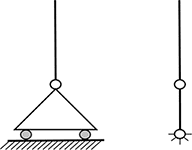 | \(u_x = 0 \\ u_y = 0\) |
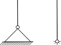 | \(u_y = 0\) |
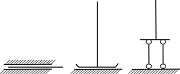 | \(u_y = 0\) \(\omega=0\) |
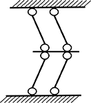 | \(\omega = 0\) |
In the table above, external constraints to the ground (i.e. set the value to zero) are reported, but the symbols are used also to express a fixed displacement/rotation different from zero.
Neumann Boundary Condition
In solid mechanics, the spatial derivatives of displacements are related to the strain tensor. In elasticity, the strain is proportional to the stress, hence the Neumann boundary condition refers to both imposed strains and stresses.
Since stress is also linked to external forces through Cauchy’s stress principle, the Neumann condition is also used to apply external loads. As stated in the section dedicated to Neumann boundary conditions, the homogeneous condition is naturally satisfied, so “free” boundaries may not be modeled explicitly.
Robin Boundary Condition
It is used to model the mechanical impedance of a structure, i.e., how much it resists motion when subjected to a harmonic load.
Fluid Mechanics
Dirichlet Boundary Condition
In computational fluid mechanics, the classical Dirichlet boundary condition consists of the value of velocity and/or pressure to be taken by a certain set of nodes. It is common to refer to some sets of b.c. according to the following terminology:
- Slip boundary condition: the velocity normal to the boundary is set to zero, while the velocity parallel to the boundary is left free
- No-slip boundary condition: both the velocity normal to the boundary and the velocity parallel to the boundary are set equal to zero.
At least one homogeneous B.C. on the pressure (i.e. \(p=0\)) has to be imposed as a reference for open domains, for instance, in the highest boundary of the air domain.
Neumann Boundary Condition
Constraints on the derivative of velocity or pressure fields are mainly used in two cases. The first case is the application of a symmetry plane:
$$ \cfrac{\partial u}{\partial n} = 0 \tag{10}$$
Since this condition is always applied in addition to a Dirichlet B.C., it is naturally satisfied. The second application is the modeling of wall friction in the case when it is proportional to the strain rate:
$$ S=(\nabla u + \nabla^T u) \tag{11}$$
Robin Boundary Condition
The Robin B.C. used to describe semi-reflective walls, which partially absorb waves. It is not a very common application, and it can be used only for pressure-based models. This B.C. is mostly used for acoustic applications.
Thermodynamics
Dirichlet Boundary Condition
In thermodynamics, Dirichlet boundary conditions consist of surfaces (in 3D problems) held at fixed temperatures.
Neumann Boundary Condition
The Neumann boundary condition in thermodynamics represents the heat flux across the boundaries. The perfect insulator reflects a homogeneous condition (naturally satisfied), while all warmed and cooled boundaries are required to explicitly assign the boundary condition. This is normally the case with electronic components (inward heat flux) or external cooling spray/channel (outward heat flux).
Electromagnetism
Maxwell equations are commonly solved through a potential formulation. In this section, the (\(A,\varphi\)) formulation is considered, where \(A\) is the magnetic vector potential, and \(\varphi\) is the scalar electric potential.
Under certain conditions, the (\(A,\varphi\)) can be decoupled, and the electric potential can be computed through the Laplace equation:
$$ \Delta\varphi=0 \tag{12}$$
Dirichlet Boundary Condition
The Dirichlet boundary condition on \(\varphi\) is usually imposed on the boundary sections of the conductive domain; in the case of wires, the values on one section are normally set to zero, while a fixed value of the electric potential is fixed on the second section. The conditions on \(A\) usually constrain the magnetic field to be tangent to the external boundary, i.e. to have all the magnetic lines inside the computational domain.
Neumann Boundary Condition
In electromagnetic modeling, under certain hypotheses, \(\nabla\varphi\) is the electric current density. The imposition of a homogeneous Neumann boundary condition (i.e.\(\nabla\varphi\cdot n=0\)) means forcing the electric current to not cross the boundaries. This condition is also referred to as the “insulating boundary” and represents the behavior of a perfect insulator.
Robin Boundary Condition
It is used to model the impedance of an electric circuit, thus the opposition that a circuit presents to a current when a voltage is applied. It is also used to model the impedance of the electromagnetic wave.

References
- https://www.encyclopediaofmath.org/index.php/Sturm-Liouville_problem
- https://www.encyclopediaofmath.org/index.php/Sturm-Liouville_theory
- Cheng, A. and D. T. Cheng (2005). Heritage and early history of the boundary element method, Engineering Analysis with Boundary Elements, 29, 268–302.
- Gustafson, K., (1998). Domain Decomposition, Operator Trigonometry, Robin Condition, Contemporary Mathematics, 218. 432–437.
- Morse, P. M. and Feshbach, H. Methods of Theoretical Physics, Part I. New York: McGraw-Hill, pp. 678-679, 1953.
Last updated: August 11th, 2023
Did this article solve your issue?
How can we do better?
We appreciate and value your feedback.
What's Next
What is Transport Equation?

