What Is Heat Transfer?
Heat transfer describes the flow of heat (thermal energy) due to temperature differences and the subsequent temperature distribution and changes.
The study of transport phenomena concerns the exchange of momentum, energy, and mass in the form of conduction, convection, and radiation. These processes can be described via mathematical formulas.
The fundamentals for these formulas are found in the laws for the conservation of momentum, energy, and mass in combination with constitutive laws, relations that describe not only the conservation but also the flux of quantities involved in these phenomena. For that purpose, differential equations are used to describe the mentioned laws and constitutive relations in the best way possible. Solving these equations is an effective way to investigate systems and predict their behavior.
SimScale’s cloud-native simulation platform offers powerful tools for performing thermal analysis, allowing engineers to simulate heat transfer processes like conduction, convection, and radiation with ease and accuracy. Discover how SimScale can help streamline your thermal analysis workflows.
Heat Transfer – History
Without external work, heat will always flow from hot objects to cold ones as a consequence of the second law of thermodynamics. This transport of heat is called heat flow.
In the early nineteenth century, scientists believed that all bodies contained an invisible fluid called caloric (a massless fluid thought to flow from hot to cold objects). Caloric was assigned properties, some of which proved to be inconsistent with nature (for instance it had weight and it could not be created nor destroyed). For example, when rubbing our hands against one another, both hands get warmer even though initially they were both at a cooler temperature. If the cause of the heat was a fluid, then it would have flowed from a (hotter) body with more energy to another with less energy (colder).
Thompson and Joule showed that this theory of the caloric was wrong. Heat is not a substance as originally theorized, but rather, a form of kinetic energy at the molecular level (so-called kinetic theory). The hands rubbing together from the previous example are actually heated because the kinetic energy of motion (rubbing) has been converted to heat due to friction.
The flow of heat is happening all the time in nature between objects. Some examples are presented below:
- Heat is conducted or flows from your warm body to the cool air around you in an air conditioned room
- Buoyancy-driven motion, or convective motion, of the air will circulate in the room due to small temperature variations
- The Sun propagates or radiates heat across the vast vacuum of space around it due to its extremely high temperature
These examples highlight the three modes of heat transfer described in the next section.
The only system free from heat flow would have to be isothermal with an even energy distribution and perfectly insulated from any other surrounding system. These conditions are impossible to recreate in the real world.
Types of Heat Transfer
Heat Transfer or heat flow can take place in three forms:
- Conduction
- Convection
- Radiation.
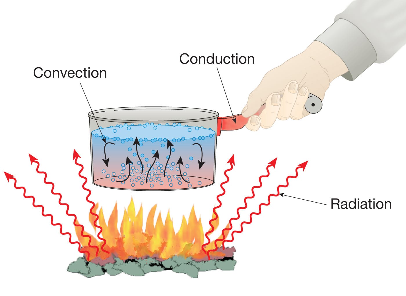
Presented below, a detailed description of each of these heat transfer methods describes the different phenomena along with their corresponding theories.
Conduction
The basis of conduction is Fourier’s law. Formulated by Joseph Fourier in 1822, he formulated a complete theory of heat conduction.
Fourier’s Law states heat flux (\(q\) resulting from thermal conduction is directly proportional to the magnitude of the temperature gradient, and that the direction of heat flow is in the negative direction relative to the temperature gradient.
$$ q = -k \frac{dT}{dx}$$
The proportionality constant, \(k\), is called the thermal conductivity with the dimensions \(\frac{W}{m*K}\), or \(\frac{J}{m*s*K}\).
The heat flux is a vector quantity. The equation above tells us that, if temperature decreases with spatial \(x\) vector, \(q\) will be positive i.e. it will flow in the positive \(x\)-direction. If \(T\) increases with \(x\), \(q\) will be negative; it will flow in the negative \(x\)-direction. In either case, \(q\) will flow from higher temperatures to lower temperatures. Equation (1) is the one-dimensional formulation of Fourier’s law. The three-dimensional equivalent form is:
$$ \overrightarrow{q} = -k \nabla T$$
where \(\nabla\) indicates the gradient.
Fourier’s law can also be expressed in a simple scalar form:
$$ q = k \frac{\Delta T}{L}$$
where \(L\) is the spatial length in the direction of heat flow and \(q\) and \(\Delta T\) are both written as positive quantities.
The thermal conductivity of gases can be understood by imagining the gas molecules as small particles. These molecules move through thermal movement from one position to another as can be seen in the picture below:
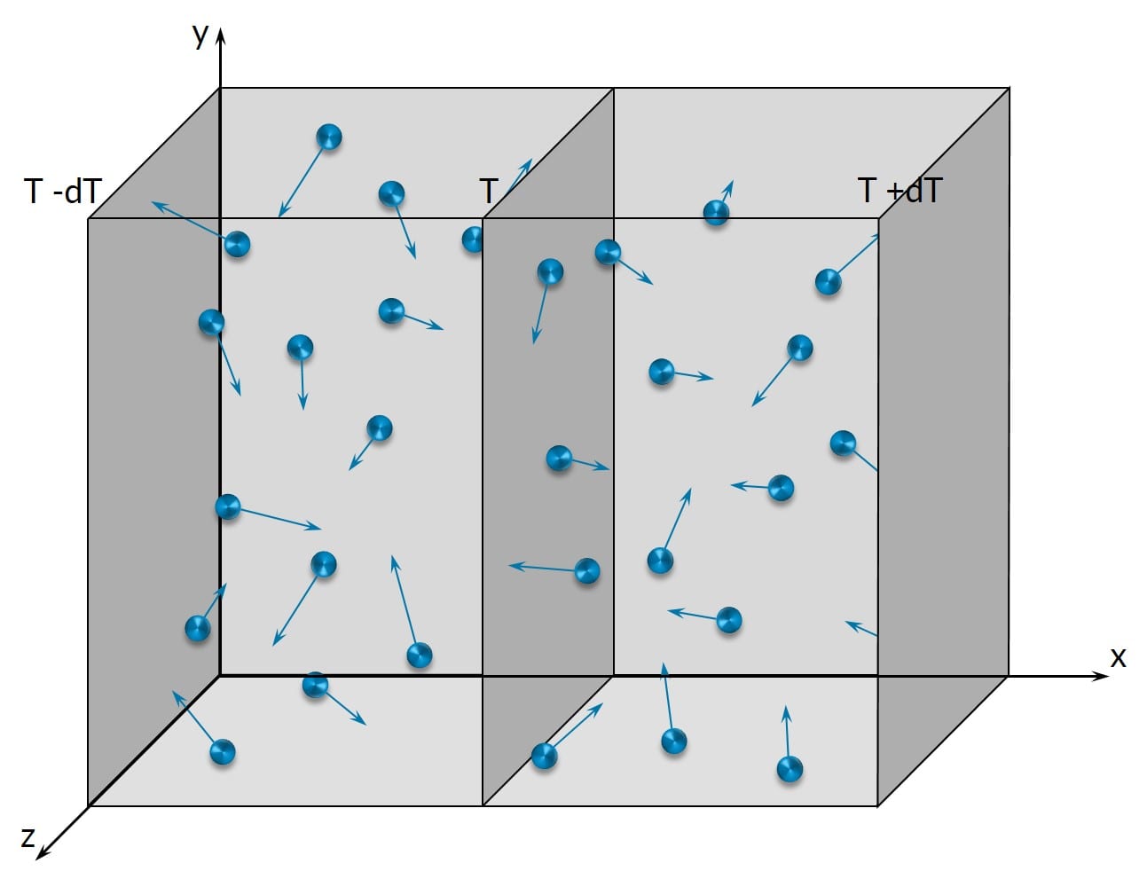
The internal energy of the molecules is transferred by impact with other molecules. Areas with low temperatures, therefore lower internal thermal energy, will absorb heat from molecules of high temperatures. The thermal conductivity can be explained with this imagination and be derived with the kinetic theory of gases [1]:
$$ T = \frac{2}{3} \frac{K}{N k_B}$$
which states that “the average molecular kinetic energy is directly proportional to the absolute temperature for an ideal gas”\(^5\). The thermal conductivity is independent of the pressure and increases with the root of the temperature.
Heat transfer via conduction in solid matter is more straightforward. In nonmetallic components, heat transfers via lattice vibrations (Phonon). The thermal conductivity transferred by phonons also exists in metals, but the more dominant form of conducted heat is via the high-conductivity electrons.
The low thermal conductivity of insulating materials like polystyrene or glass wool is based on the principle of low thermal conductivity of air (or any other gas). The following table lists some of the commonly used elements/materials and their thermal conductivities:
| Material | Thermal conductivity \(W/(m.K)\) |
| Oxygen | 0.023 |
| Steam | 0.0248 |
| Polystyrene | 0.032-0.050 |
| Water | 0.5562 |
| Glass | 0.76 |
| Concrete | 2.1 |
| Steel high-alloyed | 15 |
| Steel unalloyed | 48-58 |
| Iron | 80.2 |
| Copper pure | 401 |
| Diamond | 2300 |
Analogous definitions
Heat Transfer: Heat flux density \(\propto\) grad T (Thermal conductivity)
Diffusion: Partial current density \(\propto\) grad x (Diffusion coefficient)
Electric lead: Current density \(\propto\) grad \(U_{el}\) (Electric conductivity)
Convection
Convection is another form of heat transfer related specifically to fluids. Convection is the transport of heat due to the movement of a fluid. The movement of fluid transporting heat can be the result of different situations.
Depending on how the fluid motion is initiated, we can classify convection as natural convection or forced convection. Natural convection is caused by the buoyancy effects of a fluid with a varying temperature field that is under the influence of gravity; warm fluid rises while cold fluid falls due to density difference. Forced convection is the movement of a fluid from external means such as a fan, a pump, a suction device or the wind.
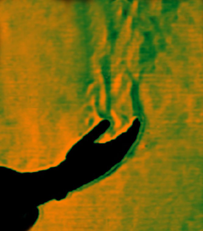
Natural convection, as the name suggests, happens all around you in nature. Sitting in an air conditioned room, your warm body transfers heat to the air you’re touching via conduction, but the warmer fluid surrounding you rises as it heats up due to its lower density; this air rising is an example of natural convection.
With forced convection, the source of the fluid movement around a body can be many things in nature or a man-made machine. However, unlike natural convection, fluid motion is not occurring due to the heating of the fluid from the body of interest. The movement of a solid material into a fluid causing fluid motion can also be considered as forced convection. A generic example is presented in the figure below, where a colder fluid with a temperature of \(T_{inf}\) is flowing from far away past a warmer body with a temperature of \(T_{body}\):
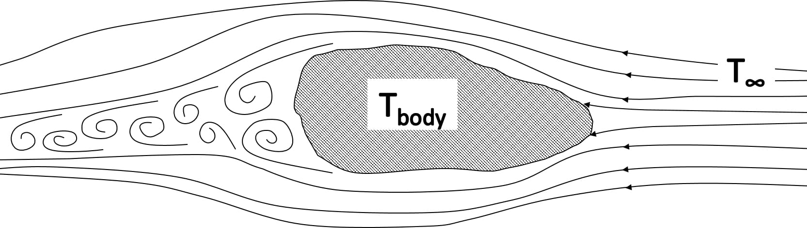
The fluid forms a thin slower-moving region called the boundary layer adjacent to the body. Heat is conducted into this layer, which is transported away and mixes into the flow downstream.
Isaac Newton (1701) considered the convective process and suggested a simple formula for the cooling:
$$ \frac{dT_{body}}{dt} \propto T_{body} – T_\infty$$
where \(T_\infty\) is the temperature of the oncoming fluid. This expression proposes that energy is flowing away from the body\(^1\).
The steady-state form of Newton’s Law of cooling defining free convection is described by the following formula:
$$ Q = h(T_{body} – T_\infty)$$
where \(h\) is the heat transfer coefficient. This coefficient, when expressed in dimensionless form, defines the Nusselt number (Nu). It can be denoted with a bar \(\overline{h}\) which indicates the average over the surface of the body. \(h\) without a bar denotes the “local” values of the coefficient.
Natural convection can create a noticeable temperature difference in a building or a room. We recognize this because certain parts of the house are warmer than others. Forced convection creates a more uniform temperature distribution and therefore a comfortable feeling throughout the entire home. This reduces cold spots in the house, reducing the need to crank the thermostat to a higher temperature\(^3\).
Radiation
Radiation is the phenomenon of energy transmission or propagation from one body to another irrespective of the presence (or lack thereof) of a medium between the two bodies. This is in contrast of conduction or convection, where the heat is transmitted within or through a body.
All bodies, fluid or solid, constantly emit energy via electromagnetic radiation. The intensity of such energy flux depends on several characteristics of the body. Thermal radiation, an instance of radiation, specifically describes the transmission of heat energy. It is dependent on the temperature of the body and the body’s surface characteristics.
Very often, radiant heat transfer from relatively cooler bodies that you may often be in contact with can be neglected in comparison to convection and conduction. Heat transfer processes happening at high temperature involve a significant fraction of radiation-based heat transfer.
Electromagnetic radiation can be seen as a stream of photons, each traveling in a wave-like pattern, moving at the speed of light and carrying energy. Electromagnetic radiation can transmit energy across a vacuum where there is no matter. Different electromagnetic radiations are categorized by the energy of the photons in them. It is important to keep in mind that if we talk about the energy of a photon, the behavior can either be that of a wave or of a particle called the “wave-particle duality” of light.
The electromagnetic (EM) spectrum: This spectrum is the range of all types of electromagnetic radiation. Simply put, radiation is energy traveling and spreading out like photons being emitted by an energy source in various EM forms such as visible light, radio waves, X-Rays, gamma-rays, microwaves and infrared light\(^3\).
Each instance of radiant energy has a wavelength, \(\lambda\) and a frequency, \(\nu\), associated with it. The relation the between the EM radiative energy, wavelength, \(\lambda\) and frequency, \(\nu\), can be described by the following formulas:
$$ \lambda = \frac{c}{\nu}$$
and energy equals Planck’s constant times the frequency, or
$$ E = h*\nu$$
where \(h\) is Planck’s constant \((6,626 070 040 * 10^{-34} Js )\).
The table below shows various forms over a range of wavelengths. Thermal radiation is from 0.1-1000 \(\mu m\).
| Characterization | Wavelength |
|---|---|
| Gamma rays | 0.3 100 \(pm\) |
| X-rays | 0.01-30 \(nm\) |
| Ultraviolet light | 3-400 \(nm\) |
| Visible light | 0.4-0.7 \(\mu m\) |
| Near-infrared radiation | 0.7-30 \(\mu m\) |
| Far infrared radiation | 30-1000 \(\mu m\) |
| Microwaves | 10-300 \(mm\) |
| Shortwave radio TV | 300 \(mm\)-100 \(m\) |
A body that can emit radiation \((\dot{Q_E})\) can also reflect \((\dot{Q_R})\), transmit \((\dot{Q_T})\), and absorb \((\dot{Q_A})\) the falling radiation.
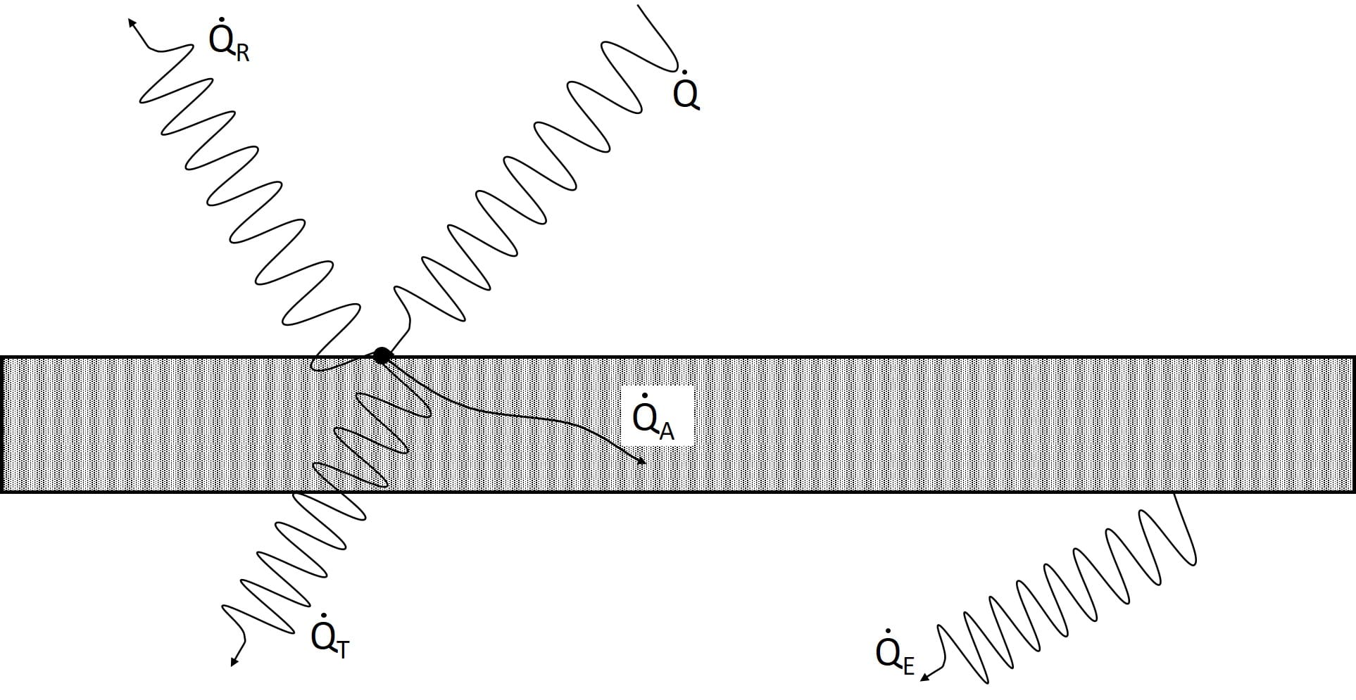
$$ \dot{Q} = \dot{Q_A} + \dot{Q_T} +\dot{Q_R}$$
$$ 1 = \frac{\dot{Q_A}}{\dot{Q}} + \frac{\dot{Q_T}}{\dot{Q}} +\frac{\dot{Q_R}}{\dot{Q}}$$
$$ 1 = \alpha^S + \tau^S + \rho^S$$
where
$$ \alpha^S : \text{Absorptance}$$
$$ \tau^S : \text{Transmittance}$$
$$ \rho^S : \text{Reflectance}$$
Different materials are commonly classified according their radiation characteristics as:
Black Body: \(\quad\) \(\alpha^S = 1\) \(\quad\) \(\rho^S = 0\) \(\quad\) \(\tau^S = 0\)
Gray Body: \(\quad\) \(\alpha^S, \rho^S\) and \(\tau^S\) uniform for all wavelengths.
White Body: \(\quad\) \(\alpha^S = 0\) \(\quad\) \(\rho^S = 1\) \(\quad\) \(\tau^S = 0\)
Opaque Body: \(\quad\) \(\alpha^S + \rho^S = 1\) \(\quad\) \(\tau^S = 0\)
Transparent Body: \(\quad\) \(\alpha^S = 0\) \(\quad\) \(\rho^S = 0\) \(\quad\) \(\tau^S = 1\)
Blackbody radiation refers to an object or system in thermodynamic equilibrium which absorbs all incoming radiation and emits energy of a characteristic, temperature-dependent spectrum. This behavior is specific of this radiating system only and is not dependent on the type of radiation which is incident upon it\(^4\).
Stefan-Boltzmann law: The thermal energy radiated by a blackbody radiator per second per unit area is proportional to the fourth power of the absolute temperature and is given by:
$$ \frac{P}{A} = \sigma T^4$$
where \(\sigma\) is the Stefan-Boltzmann constant which can be derived from other constants of nature:
$$ \sigma = \frac{2\pi ^5 k^4}{15c^2 h^3} = 5.670373 * 10^{-8} \quad Wm^{-2}K^{-4}$$
For hot objects other than ideal radiators, the law is expressed in the form:
$$ \frac{P}{A} =e \sigma T^4$$
where \(e\) is the emissivity of the object (\(e\) = 1 for ideal radiator). If the hot object is radiating energy to its colder surroundings at temperature \(T_c\), the net |link3| rate takes the form:
$$ P = e\sigma A(T^4 – T^4_c)$$
Due to the fourth power of the temperatures in the governing equation, radiation becomes a very complex, high-level nonlinear phenomenon\(^5\).
Applications of Thermal Simulation
Thermomechanical Analysis (Thermal-Structural)
Heat Transfer takes the energy balance of the studied systems into account. When investigating thermomechanical components, structural deformations, caused by the effects of thermal loads on solids can also be included. Simulating the stress response to thermal loads and failure is essential for many industrial applications. An example of an application is a thermal stress analysis of a Printed Circuit Board.
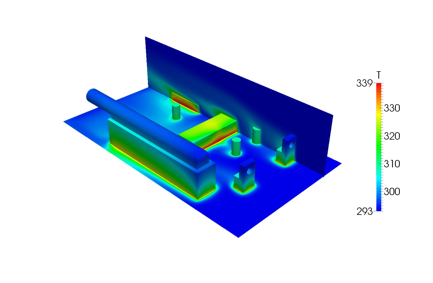
Conjugate Heat Transfer Analysis (Fluid-Solid)
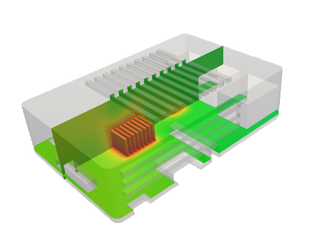
Conjugate Heat Transfer (CHT) simulations analyze the coupled heat transfer in fluids and solids. The prediction of the fluid flow while simultaneously analyzing the heat transfer that takes place within the fluid/solid boundary is an important feature of CHT simulations. One of the areas in which it can be used is for electronics cooling.
Conduction Examples
Conduction is the heat transfer from a hot object to a cold object that are in direct contact with each other. Conduction modeling allows for the direct analysis and visualization of heat transferring across the body in a given time when considering characteristics such as a body’s geometry shape and the materials’ thermal conductivity. Examples include CFL light bulbs.
Convection Examples
Convective Heat Transfer is the transfer of heat between two areas without physical contact. Convective currents occur when molecules absorb heat and start moving. Predicting both the convective cooling efficacy and the general flow stream behavior is difficult to predict without a direct simulation of the flow, requiring high computing power to obtain reliable solutions. One such application is the cooling of a Raspberry pi motherboard.
Radiation Examples
Electromagnetic waves are the source of heat transfer through radiation. They usually play a role at high temperatures. The amount of heat that is emitted via radiation depends on the surface type of the material. A general rule is that the more surface there is, the higher the radiation is. An application where simulation of radiation is used is laser beam welding.
Interested in reading more Heat-Transfer-related content?
Heat Transfer Simulation in SimScale
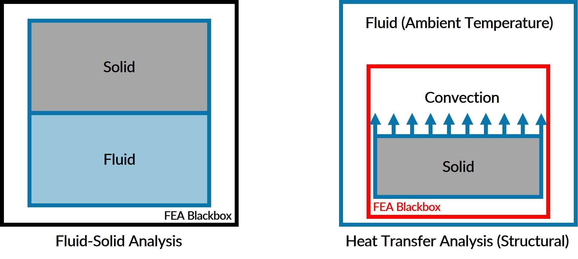
Structural Heat Transfer Software is used when:
- The fluid temperature can be assumed to be homogeneous around the solid part
- Investigating the behavior of structural components only under heating
- Investigating stress and deformation by the part caused due to heat load (thermal stress analysis)
Coupled Heat Transfer Analysis (Fluid-Solid) is used when:
- The fluid distribution around the solid needs to be studied
- Investigating the influence of the object on the fluid
- Investigating natural or forced convection
Become a SimScale member!
SimScale has the capability to solve for all three modes of heat transfer. Join SimScale today and experience powerful, multiphysics, cloud-based simulation.
Comparison of Mechanical Structural & Heat Transfer Analyses
The Structural Analysis set of simulation modules within SimScale can tackle Mechanical and Thermal problems independently or together using Finite Element Analysis (FEA) solvers. Follow a quick comparison between the two independent analyses in the table below that analogizes the problem setup between the two:
| Category | Mechanical Structural Analysis (linear static) | Heat Transfer Analysis (steady state) |
|---|---|---|
| Material properties | Young’s modulus(E) | Thermal conductivity(k) |
| Laws | Hook’s law \(\sigma=E\cdot\frac{du}{dx}\) | Fourier law \(q=-k\cdot\frac{dT}{dx}\) |
| Degree of Freedom (DOF) | Displacement (u) | Temperature (T) |
| Gradient of DOF | Strain \(\epsilon\) Stress \(\sigma\) | Temperature gradient \((\nabla T)\) |
| Similarities | Axial force per unit length: Q Cross-sectional area: A Young’s modulus: E | Internal heat generation per unit length: Q Cross-sectional area: A Thermal conductivity: k |
References
Last updated: March 16th, 2026
Did this article solve your issue?
How can we do better?
We appreciate and value your feedback.
What's Next
Numerics Background for CFD and FEA

