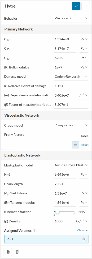
Viscoplastic Material
The viscoplastic material is available to model solid polymer materials in Nonlinear Mechanical analysis. It is based on the Parallel Rheological Framework (PRF) — an approach that combines nonlinear elasticity, viscous flow, and plasticity to accurately represent the complex mechanical behavior of polymer materials under large strains.
Standard plasticity models such as multilinear isotropic hardening or hyperelastic models alone are generally insufficient for polymers, because polymers exhibit a combination of effects that only emerge under large strains, cyclic loading, or time-dependent conditions. The Viscoplastic model is designed to capture these effects within a single material definition.
When to Use the Viscoplastic Model
Use the Viscoplastic material model when your polymer component exhibits one or more of the following behaviors under the expected loading conditions:
| Behavior | Description |
|---|---|
| Nonlinear elasticity | Stiffness that changes with the level of deformation, typical in rubbers and soft polymers |
| Mullin’s damage | Stress softening on the first loading cycle compared to subsequent cycles (also called stiffness damage) |
| Hysteresis | Energy dissipation visible as a difference between loading and unloading stress-strain curves |
| Permanent set | Residual deformation remaining after load is removed |
| Creep / viscous flow | Time-dependent deformation under sustained load |
| Strain-rate dependence | Stiffer response at higher loading rates |
Typical polymer families where this model applies include polyethylene (PE), polypropylene (PP), polycarbonate, nylon, PVC, silicone, and thermoplastic elastomers.
Viscoplastic Model Structure
The Viscoplastic model is a three-network PRF model. Each network deforms in parallel and contributes independently to the total stress response. The three networks are:
| Network | Role |
|---|---|
| Primary network | Nonlinear hyperelastic backbone; captures large-strain elastic response and optional stiffness damage (Mullin’s effect) |
| Viscoelastic network | Time-dependent viscous response; captures creep, stress relaxation, and strain-rate dependence via a Prony series relaxation model |
| Elastoplastic network | Nonlinear elastic-plastic response; captures permanent set and hysteresis through Arruda-Boyce elasticity combined with bilinear combined hardening plasticity |
Primary Network
The primary network defines the elastic equilibrium behavior of the polymer using the Yeoh hyperelastic model, which is a first-invariant-based polynomial well suited to rubbers and soft polymers across a wide strain range.
Hyperelastic Model — Yeoh
| Parameter | Symbol | Unit | Description |
|---|---|---|---|
| C10 | C₁₀ | Pa | First-order stiffness coefficient |
| C20 | C₂₀ | Pa | Second-order stiffness coefficient |
| C30 | C₃₀ | Pa | Third-order stiffness coefficient |
| Bulk modulus | \(\kappa\) | Pa | Volumetric stiffness; controls near-incompressibility |
Damage Model
An optional damage model can be added to the primary network to capture the Mullin’s effect — a reduction in stiffness observed after loading cycles. Two options are available:
| Option | Description |
|---|---|
| None | No damage; elastic response is unchanged across load cycles |
| Ogden-Roxburgh | Phenomenological damage model for Mullin’s effect; requires three scalar parameters |
When Ogden-Roxburgh is selected, the following parameters must be defined:
| Parameter | Unit | Description |
|---|---|---|
| r | — | Relative extent of damage; controls how much softening occurs |
| m | J/m³ | Dependence on deformation history |
| \(\beta\) | — | Factor applied to the maximum deviatoric strain energy in the damage criterion |
Viscoelastic Network
The viscoelastic network captures the time-dependent response of the polymer — including creep under sustained load and stress relaxation over time. The elastic part of this network shares the same Yeoh hyperelastic model as the primary network. The viscous part is defined by a Prony series relaxation model.
| Option | Description |
|---|---|
| None | No stress contribution from this network |
| Prony series | Defines creep response as a sum of exponential terms; each term is defined by a relaxation time and a Prony factor |
When Prony series is selected, enter the series as a table with one row per term:
| Column | Unit | Description |
|---|---|---|
| Relaxation time | s | Time constant for each exponential decay term |
| Prony factor | — | Amplitude of each term; must be between 0 and 1 |
Important
All Prony factors must be greater than 0 and less than 1.0, and the sum of all Prony factors must equal exactly 1.0. The simulation will not run if these constraints are violated.
Elastoplastic Network
The elastoplastic network captures the irreversible (plastic) deformation of the polymer, including hysteresis in cyclic loading and residual strain after unloading. The elastic part uses the Arruda-Boyce hyperelastic model, which is physically motivated and well-suited to lightly cross-linked polymers and thermoplastic elastomers. Plasticity is modeled with a bilinear flow rule, a von Mises yield criterion and a combined isotropic/kinematic hardening model.
| Option | Description |
|---|---|
| None | No stress contribution from this network |
| Arruda-Boyce Plastic | Nonlinear elastic-plastic model with combined hardening; requires the parameters below |
When Arruda-Boyce Plastic is selected, the following parameters are required:
| Parameter | Unit | Description |
|---|---|---|
| Nk\(\Theta\) | Pa | Stiffness of the elastic chain network; product of chain density, Boltzmann constant, and temperature |
| Chain length | — | Number of rigid links per polymer chain; controls the locking stretch |
| Yield stress | Pa | von Mises equivalent stress at which plastic flow begins |
| Hardening slope | Pa | Slope of the post-yield stress-strain curve (bilinear hardening) |
| Kinematic fraction | — | Fraction of hardening that is kinematic; value between 0 and 1 (0 = fully isotropic, 1 = fully kinematic, intermediate = combined) |
Note
For polymers that exhibit a clear Bauschinger effect (different yield stress in tension vs. compression on load reversal), a non-zero kinematic fraction is recommended. For materials without significant back-stress effects, pure isotropic hardening (kinematic fraction = 0) is a good starting point.
General Properties
To take into account the weight of the material, the density property is available.
| Property | Unit | Description |
|---|---|---|
| Density | kg/m³ | Mass per unit volume; required for all solid materials |
Last updated: May 19th, 2026
Did this article solve your issue?
How can we do better?
We appreciate and value your feedback.


