Hyperelastic Materials

Hyperelastic materials are the special class of materials which respond elastically even when they are subjected to large deformations. They show both a nonlinear material behavior as well as large shape changes. They are characterized by:

1. Can undergo large elastic deformations in order of 100 to 700% which are fully recoverable, i.e., the initial shape is recovered when load is removed.
2. Are nearly incompressible, which means that they can change their shape but overall volume remains almost constant.
3. Show a highly nonlinear stress-strain relation.
4. The material softens and then becomes stiffer again when applied to tension whereas, under compression, they have a quite stiff response.

Many polymers show hyperelastic behavior, such as elastomers, rubbers, and other similar soft flexible materials.

Hyperelastic materials are mostly used in applications where high flexibility, in the long run, is required, under the presence of high loads. Some typical examples of their use are as elastomeric pads in bridges, rail pads, car door seal, car tires, and fluid seals.

Hyperelasticity Theory

In finite element analysis, the hyperelasticity theory is used to represent the non-linear response of hyperelastic materials at large deformations. Hyperelasticity is popular due to its ease of use in finite element models. Usually, stress-strain curve data from experimental tests is used to fit the constants of theoretical models, thus approximating the material response.

The choices of hyperelasticity models which are available in SimScale platform are:

1. Neo-Hookean (first order reduced polynomial)
2. Mooney-Rivlin (first order complete polynomial)
3. Signorini (second order reduced polynomial)
4. Yeoh
5. Ogden (first, second, and third order)

Calculating the Stress-Strain Relation From Strain Energy Density Function

The stress-strain relation for hyperelastic materials is normally calculated with a strain energy density function. A brief theoretical description follows.

Consider a solid body subjected to a great deformation. A point inside the body with position $X$ with respect to the original configuration is displaced to the position $x$ in the final configuration through the displacement vector $u$:

$$x=X+u$$

The tensor of the gradient of the deformation $F$ relating the initial configuration to the final configuration is given by:

$$F=\frac{\partial x}{\partial X}=I+{\mathrm{\nabla }}_{X}u$$

The local change of volume $J$ is given by its determinant $J=det(F)$. This tensor turns out to not be the best way to describe large deformations, so the right Cauchy-Green tensor is used instead:

$$C=F^{T}F$$

This tensor is symmetrical, with its invariants given by:

$${\mathrm{I}}_C=tr(C)$$

$${\mathrm{II}}_C=\frac{1}{2}(tr(C{)}^2–tr(C^2))$$

$${\mathrm{III}}_C=det(C)$$

The third invariant ${\mathrm{III}}_C$ relates to the change in volume, and can also be written as:

$${\mathrm{III}}_C=det(F{)}^2=J^2$$

In the case of an incompressible material, $J=1$.

Of high interest for our purpose is to express the right Cauchy-Green tensor and its invariants in terms of the principal stretches ${\lambda }_i$:

$${\lambda }_i=1+{\epsilon }_i$$

$$C_{ii}={\lambda }_i^2$$

$$C_{ij}=0,i\ne j$$

$${\mathrm{I}}_C={\lambda }_1^2+{\lambda }_2^2+{\lambda }_3^2$$

$${\mathrm{II}}_C={\lambda }_1^2{\lambda }_2^2+{\lambda }_2^2{\lambda }_3^2+{\lambda }_3^2{\lambda }_1^2$$

$${\mathrm{III}}_C={\lambda }_1^2{\lambda }_2^2{\lambda }_3^2$$

where ${\epsilon }_i$ are the nominal strains in the principal directions (measured in the original configuration). Notice that the stretches ${\lambda }_i$ are the components of the gradient of deformation tensor $F$.

It is assumed that a strain energy density function $U$ exists such that the hyperelastic (second) Piola-Kirchhoff stress tensor $S$ in the material can be related to the right Cauchy-Green deformation tensor:

$$S=2\frac{\partial U}{\partial C}$$

The true stress tensor on the material is related to the second Piola-Kirchhoff stress tensor. It can be expressed (after some algebra, not shown here) in terms of the right Cauchy-Green tensor and the strain energy density function:

$${\sigma }_{ij}=-p{\delta }_{ij}+2\frac{\partial U}{\partial I_1}{C}_{ij}–2\frac{\partial U}{\partial I_2}{C}_{ij}^{-1}$$

Here, $p$ is the hydrostatic external pressure, which causes pure volumetric change, and $delt{a}_{ij}$ is the kronecker delta. Notice that due to the incompressibility assumption, the $J$ term is dropped.

For the material models available in SimScale, the strain energy density function is given by:

$$U=C_{10}(I_1–3)+C_{01}(I_2–3)+C_{20}(I_1-3{)}^2+\frac{1}{2}K(J–1{)}^2$$

$$I_1={\mathrm{I}}_c{J}^{-\frac{2}{3}}$$

$$I_2={\mathrm{II}}_c{J}^{-\frac{4}{3}}$$

$$J={\mathrm{III}}_c^{\frac{1}{2}}$$

You will find that in the user interface, the compressibility is controlled by the $D_1$ constant, given by:

$$D_1=\frac{2}{K}$$

Particular Strain Energy Density Forms of the Available Hyperelasticity Models

Before giving the appropriate material parameters to define specific hyperelastic materials, one should know the strain energy density forms of the hyperelasticity models. Following are the strain energy density forms of all the available hyperelasticity models on the SimScale platform (as mentioned above).

Neo-Hookean

With $C_{01}=C_{20}=0$ in the above formulation, one obtains the most basic form known as neo-Hookean, given by:

$$U=C_{10}(I_1–3)+\frac{1}{D_1}(J–1{)}^2$$

Mooney-Rivlin

With $C_{20}=0$ in the above formulation, one obtains the enhancement to neo-Hookean form known as Mooney-Rivlin, given by:

$$U=C_{10}(I_1–3)+C_{01}(I_2–3)+\frac{1}{D_1}(J–1{)}^2$$

Signorini

Strain energy density function for Signorini is represented as:

$$U=C_{10}(I_1–3)+C_{01}(I_2–3)+C_{20}(I_1-3{)}^2+\frac{1}{D_1}(J–1{)}^2$$

Yeoh

Strain energy potential for the Yeoh is represented as:

$$U=C_{10}(I_1–3)+C_{20}(I_2–3{)}^2+C_{30}(I_1-3{)}^3+\frac{1}{D_1}(J–1{)}^2$$

Ogden

Strain energy potential for the Ogden is represented as:

$$U=\sum _{i=1}^N\frac{{\mu }_i}{{\alpha }_i}({\lambda }_1^{\prime {\alpha }_i}+{\lambda }_2^{\prime {\alpha }_i}+{\lambda }_3^{\prime {\alpha }_i}-3)+\frac{1}{D_1}(J–1{)}^2$$

Where:

$$N=\text{Order of the Model}$$

$${\lambda }_1^{\prime },{\lambda }_2^{\prime },{\lambda }_3^{\prime }$$ are the deviatoric principal stretches ${\lambda }_p$, defined as ${\lambda }_p^{\prime }=J^{\frac{1}{3}{\lambda }_p}$

When specifying the Ogden model the user can specify the order of the model from first to third order.

Loading State

The final piece of the puzzle to be able to fully characterize the hyperelastic material is the definition of the stretches ${\lambda }_i$, which are determined by the loading state. The same material will have different behavior depending on how it is loaded, as shown in the following plot (taken from Axel Product, Inc.). In a typical test, the specimen is subjected to the desired load state, and the stress-strain relation is measured.

Uniaxial Tension

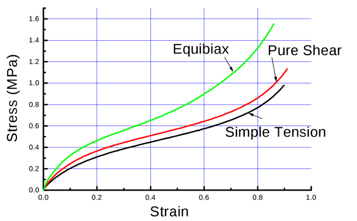
For the case of uniaxial tension loading of an incompressible material, the specimen is loaded along one axis. The stretches are given by:

$${\lambda }_1=1+\epsilon$$

$${\lambda }_2={\lambda }_3={\lambda }_1^{-1/2}$$

Equibiaxial Tension

For the case of equibiaxial tension loading of an incompressible material, the specimen is loaded along two perpendicular axes with the same magnitude. The stretches are given by:

$${\lambda }_1={\lambda }_2=1+\epsilon$$

$${\lambda }_3={\lambda }_1^{-2}$$

Pure Shear

For the case of pure shear loading of an incompressible material, the specimen is loaded in two perpendicular directions, one in tension and the other in compression. Plane strain condition is assumed, so there is no deformation in the unloaded direction. The stretches are given by:

$${\lambda }_1=1+\epsilon$$

$${\lambda }_2=1$$

$${\lambda }_3={\lambda }_1^{-1}$$

Getting Material Parameters From Experimental Data

In order to fit the material properties to the experimental stress-strain curve, one has to take into account all the relations presented above. Combining the equations, the stress is expressed in terms of the strain, and the constants of the model are determined through a least-squares fit of that function to the test data. In most of the cases, the accuracy of the fit increases with the increasing order of the model.

As an example, let us consider a stress-strain relation of an incompressible uniaxial case for a Signorini model:

$$U=C_{10}(I_1–3)+C_{01}(I_2–3)+C_{20}(I_1-3{)}^2+\frac{1}{D_1}(J–1{)}^2$$

Using the given definition for uniaxial stretches, the principal true stress can be written as:

$${\sigma }_{11}=-p+2\frac{\partial U}{\partial I_1}{\lambda }^2–2\frac{\partial U}{\partial I_2}{\lambda }^{-2}$$

And:

$${\sigma }_{22}=-p+2\frac{\partial U}{\partial I_1}{\lambda }^{-1}–2\frac{\partial U}{\partial I_2}\lambda =0$$

After subtracting to get rid of the pressure term, factoring out, and performing the derivatives we get:

$${\sigma }_{11}=2({\lambda }^2–{\lambda }^{-1})[\frac{\partial U}{\partial I_1}+{\lambda }^{-1}\frac{\partial U}{\partial I_2}]$$

$$\frac{\partial U}{\partial I_1}=C_{10}+2C_{20}(I_1–3)$$

$$\frac{\partial U}{\partial I_2}=C_{01}$$

This completes the stress-strain function that should be input to the least-square fit algorithm to determine the $C_{10},C_{01},C_{20}$ constants.

Similar expressions can also be derived for the equibiaxial tension case:

$${\sigma }_{11}=2({\lambda }^2–{\lambda }^{-4})[\frac{\partial U}{\partial I_1}+{\lambda }^2\frac{\partial U}{\partial I_2}]$$

And for pure shear case:

$${\sigma }_{11}=2({\lambda }^2–{\lambda }^{-2})[\frac{\partial U}{\partial I_1}+\frac{\partial U}{\partial I_2}]$$

Notice that due to the incompressibility condition, the $D_1$ parameter can not be estimated with this procedure. The recommendation is to give an approximate value using the elasticity relations:

$$D_1=\frac{1–2\nu }{C_{01}+C_{10}}$$

For an almost incompressible material, the value of $\nu$ is close to 0.5.

Giving Material Parameters in SimScale

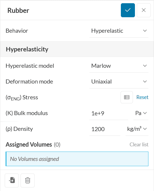
Once the material constants of a specific model are obtained from a good fit to experimental data, one can input these constants to the specified material model in SimScale under material properties:

• The provided constants can be the proper combinations of $C_{10}$, $C_{01}$, and $C_{20}$ as obtained from fitting.
• It is observed that in some cases if any of the obtained constant value is comparatively higher than the other constants then the results obtained after the simulation are not accurate.
• For the incompressible case, one can:
  • Use the recommended value for $D_1$ with $\nu$ = 0.499 as a first approximation.
  • Get more accurate results by giving smaller values to $D_1$. This will make the material closer to fully incompressible.
  • If you run into convergence issues, stop giving smaller values to $D_1$.
  • Give value to $D_1$ at least 1×10^− 10.

Last updated: September 26th, 2024