What is Electromagnetic Induction?
Electromagnetic induction, discovered by Michael Faraday in 1831, uncovers the fascinating relationship between magnetic fields and electric currents, fundamentally transforming our understanding of energy generation. The principle of electromagnetic induction signifies that a changing magnetic field can induce an electric current in a conductor, eliminating the necessity for a battery to produce a current.
At first glance, magnets captivate us with their mysterious qualities and invisible forces. However, it is truly remarkable to realize that these seemingly ordinary objects are intricately interconnected with many aspects of the technologies that propel and shape our daily lives.
Imagine a bustling city, its streets illuminated by countless streetlights, factories humming with productivity, and homes buzzing with appliances. Ever wondered how all this electrical power is generated? In a nutshell, it all stems from the concept of electromagnetic induction.
SimScale is launching a brand new simulation category that enables users to conduct electromagnetic simulations in the cloud. Initially, the focus will be on magnetostatics simulations, but over time, the electromagnetics simulation capabilities will gradually expand to encompass a wide range of industrial applications.
Throughout this article, we will delve deeper into the interesting world of electromagnetic induction, exploring the principles, mechanisms, and real-world applications that make it a cornerstone of modern technology.
Fundamentals of Magnetic Fields
In order to grasp the concept of electromagnetic induction, it is helpful to establish a basic understanding of the nature of magnetic fields. Magnetic fields differ from electric fields and can be more challenging to make sense of.
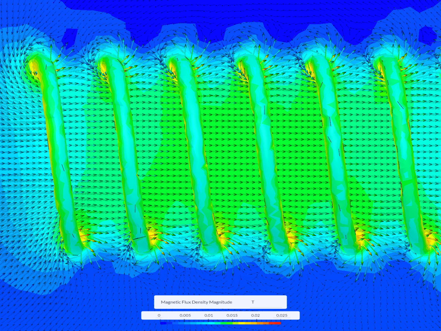
In the field of electromagnetics, the term “magnetic field” refers to two vector fields that are closely connected and represented by the symbols \(B\) and \(H\).
\(B\) is the magnetic flux density and has a unit of Tesla \([T]\), while \(H\) is the magnetic field strength and has a unit of \([A/m]\).
Unlike electric fields that stem directly from individual charges, the magnetic field arises in a nuanced manner due to the absence of magnetic charges. Additionally, the absence of magnetic charges results in the magnetic field lines (more precisely, the magnetic flux density \(B\)) always forming closed loops devoid of any beginnings or endings. Here, the magnetic field refers to the magnetic flux density \(B\).
In the absence of magnetic charges, the generation of magnetic fields occurs through indirect means. It is an inherent principle in nature that the motion of electric charges, including moving electrons, gives rise to magnetic fields. This applies to electrical currents flowing through wires, as currents involve the collective movement of numerous electrons. Consequently, a continuous (DC) current passing through a wire generates a magnetic field that forms a circular pattern around the wire, as illustrated in Figure 1.
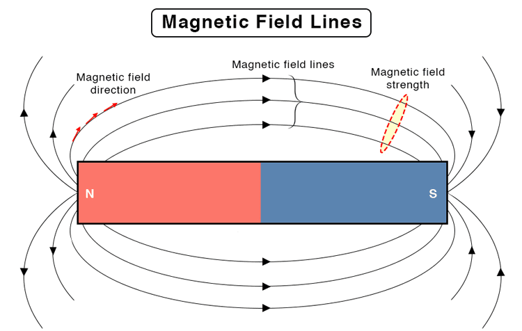
Magnetic field lines possess distinct properties that aid in understanding the behavior of magnetic fields \(B\). These lines form closed and continuous curves, meaning they create a loop without any breaks. The density of the magnetic field lines indicates the strength of the magnetic field. When the lines are crowded or closely spaced, it signifies a strong magnetic field. Conversely, as the distance from the object increases, the density of the lines decreases, reflecting a weaker magnetic field.
Moreover, magnetic field lines never intersect or cross each other. If such an intersection were to occur, the tangent at the point of intersection would indicate different directions, which contradicts the nature of magnetic fields. This is only true at points where the field is not zero.
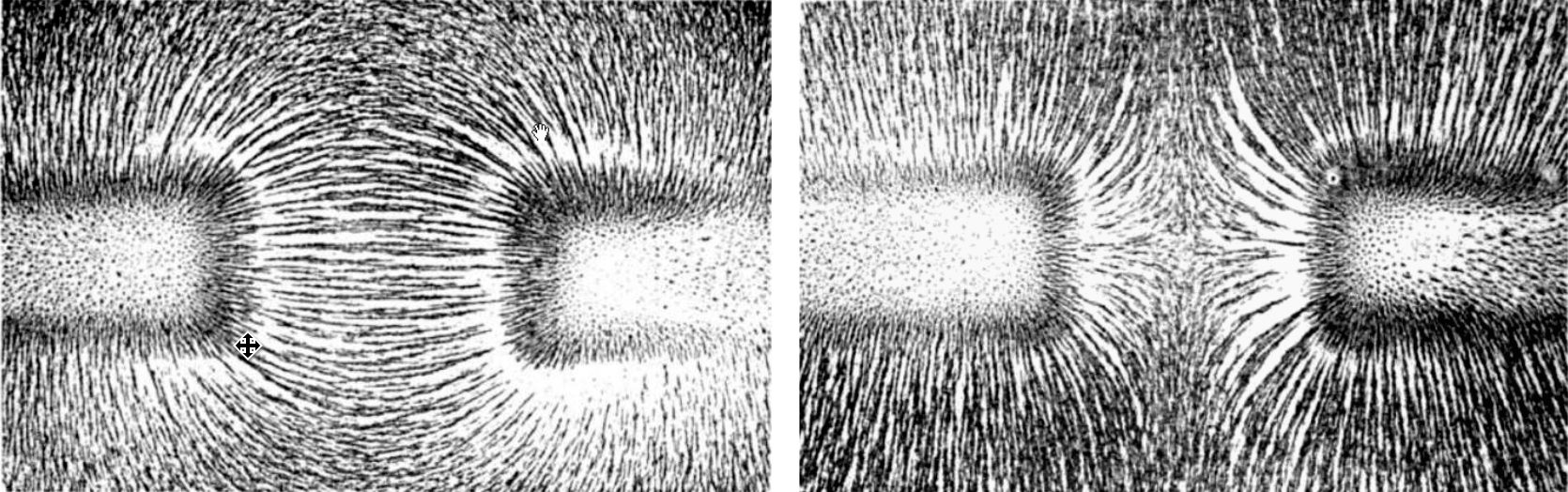
Left: Different magnetic poles configuration leading to an attracting magnetic field; Right: Similar magnetic poles configuration leading to a repelling magnetic field.\(^2\)
Faraday’s Law of Electromagnetic Induction
Faraday’s Law of Induction stands as a cornerstone in the field of electromagnetism, providing a profound understanding of the relationship between magnetic fields and electrical currents. This principle was discovered by the eminent scientist Michael Faraday in 1831.
At its core, Faraday’s Law of Induction states that an electromotive force (EMF) is induced in a circuit whenever relative motion exists between a conductor and a magnetic field, and the magnitude of this EMF is proportional to the rate of change of the magnetic flux. Therefore, we understand that a magnetic field can be used to create a voltage (which is an EMF). If a closed circuit exists, then a current will flow in that circuit.
Magnetic Field Around a Conducting Wire
Let’s explain this law by starting with a simple example of a current flowing through a conducting wire. In the previous section, we understood that a magnetic field is produced around a conducting wire when an electric current is flowing through it. This phenomenon in particular is what’s known as Ampere’s law.
If this wire is wound into a coil, the magnetic field around that coil is significantly intensified. This is because by adding more loops to a coil, the magnetic fields generated by each individual loop combine to create a focused magnetic field along the center of the coil. This interaction is illustrated in the figure below, which depicts a loosely wound coil.
As the coil is wound tighter, the magnetic field becomes more uniformly distributed along the entire length of the coil. The magnetic field intensity of a coil is enhanced not only by increasing the current but also by augmenting the number of loops within the coil.
When a coil of wire is long and straight, it is referred to as a solenoid and can generate a magnetic field that closely resembles the uniformity of a bar magnet.
Electromagnetic Induction in Action
Now, what if we were to remove the electrical current from the coil and replace the empty core with a bar magnet positioned inside the coil of wire? As we manipulate the position of this bar magnet, pulling it inwards and pushing it outwards, the physical movement of the magnetic flux within the coil would induce an electric current within it.
Similarly, if we were to fix the bar magnet in place and, instead, move the coil back and forth within the magnetic field, an electric current would be generated within the coil. Hence, by either moving the coil or changing the magnetic field, we can induce both voltage and current within the coil. This phenomenon is referred to as Electromagnetic Induction.
For added clarity, remember that there is a magnetic field associated with the bar magnet; the lines of the magnetic field pass through the coil. In other words, there is a magnetic flux across the coil. The change of this magnetic flux which can be done either by moving the magnet or the coil is what induces an EMF and, hence, a current in the coil.
Figure 5 below demonstrates this process very clearly by means of a galvanometer. A galvanometer is an electromechanical device used for measuring electric current.
Through the connection of an electrical wire to this instrument, it possesses the capability to detect the presence or absence of electric flow within the wire. In the absence of current, the galvanometer’s needle will move towards the left, while the occurrence of an electric current will prompt a movement towards the right side of the scale.
Here, the wire is wrapped around an iron core, and a magnet is moved in and out of the iron core. Through this movement, the magnetic flux through the electrical wire is changing, and a current is induced in the wire. When the magnet reaches a halt, the galvanometer needle does not move as there is no current in the wire. In essence, it does not matter whether the magnet or the iron core is the moving object. As long as the magnetic flux through the wire is changing, an EMF is induced in the wire leading to a current that will be detected by the galvanometer.
Factors Affecting the Strength of the Induced EMF
The question now is what affects the strength of the induced EMF and, in the case of a closed circuit, the amount of current. There are three main influencing factors:
- Increasing the number of turns in the coil: By adding more turns of wire to the coil, the total induced electromotive force (EMF) amplifies. This occurs because each individual turn of the coil contributes to the overall EMF, resulting in a cumulative effect. For instance, if there are 100 turns in the coil, the induced EMF will be 100 times larger compared to a single piece of wire due to the increased magnetic field interactions.
- Increasing the speed of relative motion between the coil and the magnet: When the coil of wire moves at a higher speed through a magnetic field, the rate at which it cuts the magnetic field lines increases. As a result, the flux linkage, which determines the induced EMF, intensifies. Thus, a faster motion of the coil enhances the efficiency of electromagnetic induction, leading to a higher induced EMF.
- Enhancing the strength of the magnetic field: If the magnetic field through which the coil of wire moves becomes stronger, the number of magnetic field lines that the coil intersects also increases. This elevated magnetic field density translates into a greater flux linkage, resulting in a higher induced EMF. By manipulating the strength of the magnetic field, we can effectively control the magnitude of the induced EMF through electromagnetic induction.
Explore Electromagnetics in SimScale
Lenz’s Law of Electromagnetic Induction
Lenz’s law is a fundamental principle in electromagnetic induction that helps us understand the direction of the induced current when there is a change in the magnetic field. This law, proposed by the Russian physicist Heinrich Lenz in 1834, is based on the principle of conservation of energy and sheds light on the relationship between magnetic fields and induced currents.
The Direction of Induced Current
According to Lenz’s law, the induced current always flows in a direction that opposes the change in the magnetic field that caused it. In other words, the induced current creates a magnetic field that acts in the opposite direction to the original magnetic field. This behavior can be attributed to the interaction between the magnetic field and the charged particles in the conductor.
To visualize this concept, imagine a scenario where a magnet is moved towards a loop of wire, similar to the example in Figure 5 from the previous section. As the magnet approaches the loop, the magnetic flux passing through the loop increases. According to Lenz’s law, the induced current in the loop will flow in such a way that it produces a magnetic field that opposes the incoming magnetic field. This opposing field helps to slow down the change in the magnetic flux and conserve energy.
Similarly, if the magnet is moved away from the loop, the magnetic flux passing through the loop decreases. Lenz’s law dictates that the induced current will now flow in the opposite direction to generate a magnetic field that resists the decreasing magnetic flux. This opposing field helps to maintain the overall magnetic flux and uphold the principle of energy conservation.
Energy Conservation in the Context of Electromagnetic Induction
We speak of energy conservation in this context, but we should first really understand where that energy in the magnetic field is actually coming from. In short, the energy of the magnetic field comes from the current that caused it.
Consider a basic electrical circuit, where a power source supplies energy to a resistor through a wire. Once the system reaches a steady state, a constant magnetic field forms around the wire, which stores the transferred energy.
This energy transfer follows the principles of Lenz’s law, which acts as the magnetic counterpart to Newton’s third law. Lenz’s law can be summarized as the generation of an opposing electric field whenever a change occurs in the magnetic field. This opposing electric field, often called back-EMF (back electromotive force), arises to counteract the alteration of the magnetic field.
Building upon the given scenario, when the power is activated, the wires generate a magnetic field that begins to form around them. As this magnetic field undergoes a transition from zero to a non-zero value, Lenz’s law dictates the generation of an electric field that counteracts this change.
This electric field becomes apparent in the circuit as voltage. The opposing voltage persists until the current reaches its ultimate steady-state value. Consequently, the current cannot undergo an instantaneous change but gradually progresses from zero to its final magnitude over a specific time interval.
Additionally, as the current undergoes an increase, there exists a voltage drop across the wires. The presence of voltage and current implies power dissipation. While real-world wires inherently experience resistive losses, such as heating, we will disregard these losses in this particular example.
The power encountered in this scenario corresponds to the energy transferred into the magnetic field surrounding the wires. Similar to the energy required to accelerate a car, the energy required to increase the rate of change in a circuit, namely the current, must be considered.
Lenz’s law can be perceived as a mechanism through which nature ensures energy conservation. Energy conservation is a fundamental principle, and Lenz’s law elucidates how this principle is upheld in the realm of magnetic fields.\(^4\)
Eddy Currents
Eddy currents are induced circulating currents that arise in conductive materials when exposed to changing magnetic fields. These swirling currents, named after the eddies seen in flowing water, are an intriguing manifestation of the interplay between magnetic fields and conductors.
When a conductor, such as a metal plate is subjected to a varying magnetic field, the magnetic flux passing through the conductor changes over time. As a result, according to Faraday’s law of electromagnetic induction, an EMF is induced in the conductor, giving rise to eddy currents.
These currents circulate within the conductor in closed loops, creating localized magnetic fields that oppose the change in the original magnetic field. In general, any factor that leads to variations in the strength or orientation of a magnetic field can give rise to the occurrence of eddy currents within a conductor.
Similar to any electric current flowing through a conductor, an eddy current generates its own magnetic field. According to Lenz’s Law, the direction of the induced current, such as an eddy current, is such that the resulting magnetic field opposes the change in the magnetic field that gave rise to it.
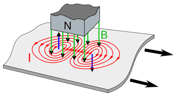
Figure 6 illustrates the interaction between a moving conductive metal sheet and a stationary magnet. As the sheet approaches the left edge of the magnet, it encounters an increasing magnetic field, leading to the generation of counter-clockwise eddy currents. These eddy currents create their own magnetic fields that oppose the external magnetic field, giving rise to a phenomenon known as magnetic drag or magnetic damping.
As the conductive metal sheet moves away from the edge of the magnet, it exits the magnetic field, causing a change in the field’s direction. This change induces clockwise eddy currents within the sheet, which generate a magnetic field that points downwards. Consequently, this downward magnetic field attracts the external magnet, resulting in the production of drag.\(^5\)
Practical Implications of Eddy Currents
Eddy currents give rise to various effects, some of which can be advantageous, while others may result in undesired consequences. One significant effect is the generation of heat within the conductor due to the resistance encountered by the eddy currents. This phenomenon is commonly observed in applications such as induction heating, where controlled eddy currents are exploited to heat objects for various industrial processes.
However, in certain scenarios, eddy currents can cause energy losses and undesirable effects. For instance, in transformers and electric motors, where energy dissipation as heat due to eddy currents is a waste of energy in the overall process.
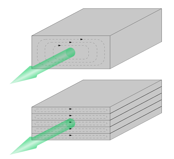
To minimize power losses, transformers often employ a laminated core, as depicted in Figure 7 below. Unlike a solid core, the laminated core consists of thin steel laminations with a nonconductive coating on their surfaces. This configuration prevents eddy currents from traversing between laminations, limiting them to flow within each individual lamination. By confining the eddy currents to a smaller area, their magnitude is significantly reduced, resulting in decreased energy dissipation within the core.
If you are coming from a CFD background, this is very similar to the concept of vortex shedding and how it is desired to break the vortices (eddies) to reduce their impact on the structure of interest.
Moreover, eddy currents can have implications in magnetic braking systems, where their generation within a rotating metallic disk or cylinder creates a drag force that slows down the motion. This principle is utilized in devices like magnetic brakes and eddy current dampers.
Applications of Electromagnetic Induction
Understanding the relationship between magnetic fields and electrical currents allowed scientists and engineers to develop various devices and systems that harness electromagnetic induction for diverse purposes.
Some of those applications are:
- Power generation
- Electrical Transformers
- Induction Motors
- Wireless Charging
- Magnetic Levitation
Electromagnetic Induction in Transformers
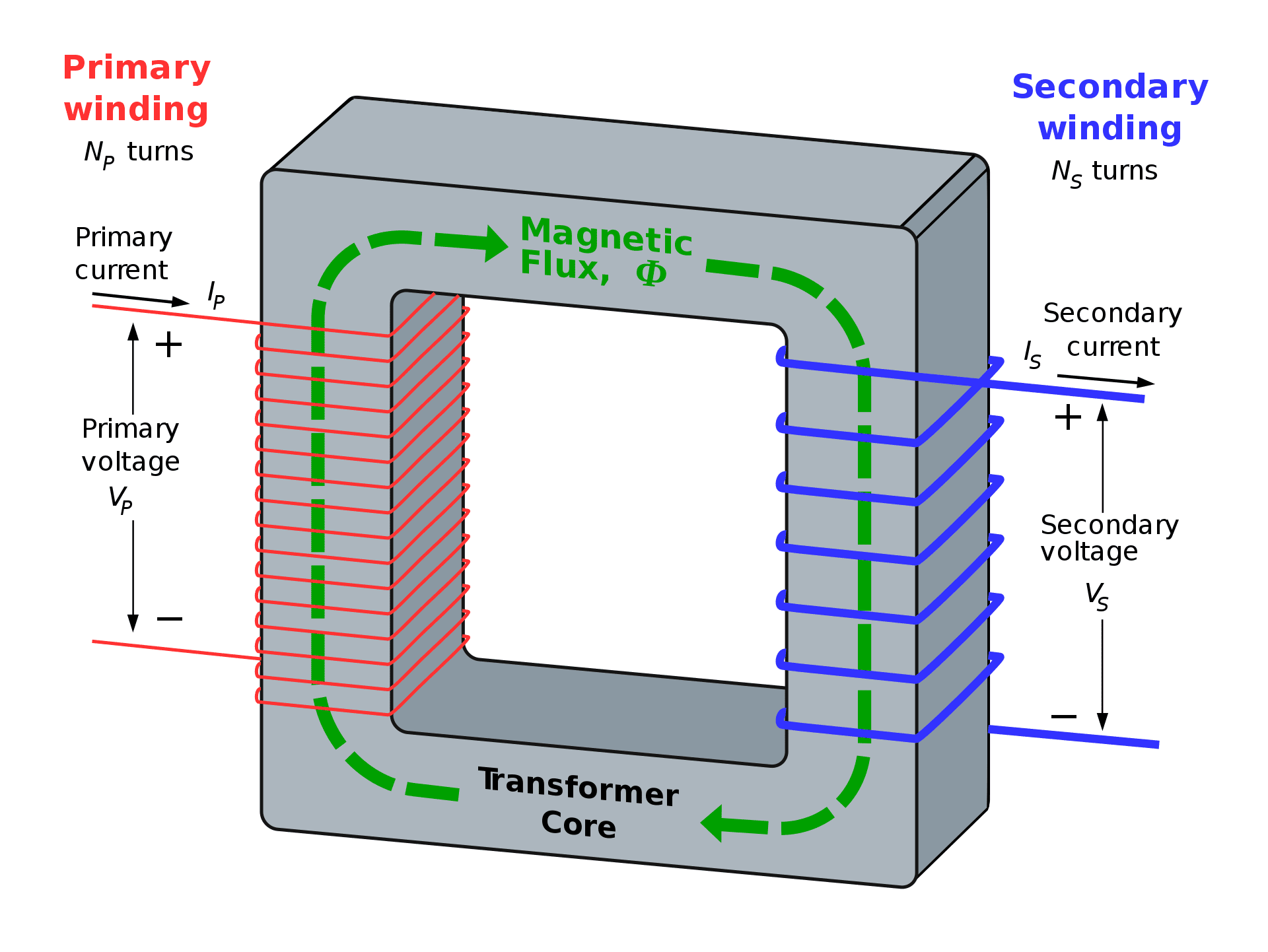
One of the most significant applications of electromagnetic induction is found in transformers. Transformers play a crucial role in electrical power distribution systems, allowing efficient transmission of electricity over long distances and enabling voltage transformation. The working principle of a transformer is based on mutual induction between two coils of wire, known as the primary and secondary coils.
A transformer functions under the law of energy conservation, which states that energy can neither be created nor destroyed, only transformed. Therefore, a transformer does not make electricity, it merely changes the voltage to suit the needs of the user. Transformers accomplish this change in voltage through the process of electromagnetic induction.
When an alternating current (AC) flows through the primary coil, it creates a varying magnetic field around it. This changing magnetic field induces a voltage in the secondary coil through electromagnetic induction.
By adjusting the number of turns in each coil, transformers can step up or step down the voltage level according to the requirements of the electrical grid. This capability ensures that electrical energy can be transmitted at high voltages over long distances, reducing power losses, and it can then be transformed to lower voltages suitable for consumer use.
References
- https://www.sciencefacts.net/magnetic-field-lines.html
- https://energyeducation.ca/encyclopedia/Magnetic_field
- https://www.nde-ed.org/Physics/Magnetism/electricitymagnet2.xhtml
- https://www.sciencedirect.com/book/9780750674034/electromagnetics-explained
- https://www.magcraft.com/blog/what-are-eddy-currents
- https://www.semanticscholar.org/paper/Effects-of-burrs-on-a-three-phase-transformer-core-Mazurek/b93536127d7c32e8ebdeca5b8f324a69ec25c6df
- https://www.galco.com/comp/prod/trnsfmrs.htm
Last updated: February 20th, 2026
Did this article solve your issue?
How can we do better?
We appreciate and value your feedback.
What's Next
Induction Heating: Basics, Advantages, & Applications

