Documentation
Magnetostatics is a model for describing magnetic fields in the case of stationary (temporally constant) or approximately constant currents and magnetizations. The model is the basis of one type of electromagnetic simulation. Many questions about important applications, from magnetic storage devices to large motors, are well answered by using this model, which is why we will take a closer look at it in this article.
Electrically charged objects and objects carrying a current (i.e., flowing charges) influence each other without touching. To explain this influence without direct contact, we use the concept of the electromagnetic field: Each point \(\mathbf{x}\) and time \(t\) is assigned a vector \(\mathbf{E}(\mathbf{x},t)\) and a vector \(\mathbf{B}(\mathbf{x},t)\). \(\mathbf{E}\) is the electric field strength and \(\mathbf{B}\) is the magnetic induction, sometimes also called magnetic flux density.
If \(\mathbf{E}\) and \(\mathbf{B}\) are known, forces (per volume) on charge density distributions \(\rho\) and flowing charges represented by the current density vector \(\mathbf{J}\) can be calculated by means of the Coulomb-Lorentz force law.
In other words, the Coulomb-Lorentz force affects charged particles, whether they are still or in motion, and is influenced by both electric fields from stationary charges and magnetic fields from moving charges or changing electric fields. It plays a crucial role in controlling how charged particles move in electromagnetic situations.
\begin{equation} \mathbf{f} = \rho\, \mathbf{E} + \mathbf{J} \times \mathbf{B}\, \end{equation}
However, in the presence of matter, \( \rho\) and \(\mathbf{J}\) are not easily available. One proportion of them consists of microscopic charges and currents within matter which develop as a reaction of the matter to an electromagnetic field acting from outside. The charge carriers involved in this have only a very small radius of action. The other proportion consists of the so-called free charges and current. An example of a free current is electrons flowing in a conductor. For the free charges and currents, it is easier to make a-priori assumptions on their distribution and quantification.
For this reason, macroscopic (i.e., spatially averaged) fields are used to calculate technical applications. The effect of the microscopic charge displacements and currents is described by the effect of the polarization \( \mathbf{P} \) and magnetization \( \mathbf{M} \), respectively.
Furthermore, two auxiliary quantities \( \mathbf{D} \) (called dielectric displacement) and \( \mathbf{H} \) (called the magnetic field strength) are introduced, which are caused only by free charges \( \rho_{\textrm{free}} \) and currents \( \mathbf{J}_{\textrm{free}} \). The (now averaged) fields \(\mathbf{E}\) and \(\mathbf{B}\) are thus split into two parts: A part originated by free charges and currents and a part that is generated by the locally bound microscopic sources:
\[ \mathbf{B} = \mu_0\, (\mathbf{H} + \mathbf{M}) \]
\[ \mathbf{E} = \epsilon_0^{-1}\, \mathbf{D} – \mathbf{P} \]
The constants \( \mu_0 \) and \( \epsilon_0 \) are the permeability and permittivity of free space, respectively. In SI units, we have \(\mu_0 = 4\pi \times 10^{-7}~\mathrm{\frac{V\,s}{A\,m}}\) and \(\epsilon_0 = \frac{1}{\mu_0c^2} \approx 8.85 \times 10^{-12}~\mathrm{\frac{A\,s}{V\,m}}\), where \( c \) is the speed of light in a vacuum.
Then the (macroscopic) Maxwell’s equations tell us how the electromagnetic field reacts to the presence and flow of free charges:
\begin{align} \nabla\times\mathbf{H} &= \mathbf{J}_\textrm{free} + \frac{\partial\mathbf{D}}{\partial t}\,,\\ \nabla\times\mathbf{E} &= -\frac{\partial\mathbf{B}}{\partial t}\,,\\ \nabla\cdot\mathbf{D} &= \rho_\textrm{free}\,,\\ \nabla\cdot\mathbf{B} &= 0\, \end{align}
The first equation is called Maxwell Ampere law, the second equation is called Faraday’s law, and the two remaining equations are called the electric Gaussian law and magnetic Gaussian law, respectively.
These equations will be completed by constitutive equations relating \( \mathbf{B} \) with \( \mathbf{H} \), and \( \mathbf{E} \)with \( \mathbf{D} \) and \( \mathbf{J} \). With the help of these macroscopic laws, detailed bookkeeping of the microscopic charges and currents is no longer necessary. For simple materials, the following applies approximately:
\begin{align} \mathbf{D} &= \epsilon\, \mathbf{E}\\ \mathbf{B} &= \mu\, \mathbf{H}\\ \mathbf{J} &= \sigma\, \mathbf{E}\; \text{(Ohm’s law)} \end{align}
where \(\sigma\) is the electric conductivity, \( \epsilon = \epsilon_{0} \, \epsilon_{r} \) and \( \mu= \mu_{0} \, \mu_{r} \), where with dimensionless constants \(\epsilon_r\) (the relative permittivity) and \(\mu_r\) (the relative permeability) depend on the material. For vacuum and approximately for air, we have \( \mu_{r} = \epsilon_{r} = 1 \).
Note that this is only the simplest case. In general, \(\epsilon\) and \(\mu\) can be tensors and depend on \( \mathbf{E} \) and \( \mathbf{B} \) respectively, as we will see in a following section.
Maxwell’s Equations describe any electromagnetic phenomena, from antennas and wave propagation of mobile phones to large electric generators and high-voltage cables. However, sometimes it is recommended to simplify Maxwell’s equations if it leads to a faster and easier solution and/or less necessary input data.
If we assume that all time derivatives in Maxwell’s equations become zero (i.e., a static limit), the magnetic and electric fields are completely decoupled from each other and can be solved separately.
The model for the static electric field will be the topic of a subsequent SimWiki article. Here, we focus on the magnetic field. The remaining equations read:
\begin{align} \nabla\times\mathbf{H} &= \mathbf{J}_\textrm{free} \,,\\ \nabla\cdot\mathbf{B} &= 0 \end{align}
completed by the constitutive equation
\[ \mathbf{B} = \mu\, \mathbf{H} \] or \[ \mathbf{B} = \mu_0\, (\mathbf{H} + \mathbf{M}) \]
with \( \mathbf{M} \) being the magnetization. The equations listed in this section are called the magnetostatic model.
This model is applicable when:
The phenomena that this model can describe are called magnetostatic phenomena.
The magnetostatic model can be used, for example, for the calculation of an electromagnet and other applications mentioned in the “Applications in Magnetostatics” section. Among other things, it cannot be used for induction phenomena (e.g., induction cooker) or wave propagation (e.g., antennas), in which case the terms omitted in Maxwell’s equations would play a role.
In magnetostatics, we only deal with the magnetic field and how matter interacts with it, i.e., with what kind of magnetization \( \mathbf{M} \) matter reacts to an external field.
There are three different types of magnetism:
Only Ferromagnetism is of high technical relevance. Therefore, we explain the first two very briefly below and focus more on ferromagnetism.
Diamagnetism is based on a quantum mechanical effect. However, the phenomenon can be imagined as a reaction of the orbital electrons, which build up a counter-field to an external field as micro-current loops and, thus, weaken the external field inside the diamagnetic body.
Magnetic field lines, which are curves tangential to the magnetic field at any point, are thus forced out of the material. Unlike paramagnetism and ferromagnetism, repulsion occurs.
In principle, all materials exhibit diamagnetism, even ones typically considered non-magnetic, like water. Diamagnetism is a weak effect, as indicated by the relative permeability \( \mu_r \) being slightly less than one (the value for a vacuum). Here, slightly less than one means that the magnetic effect on such materials is very small. For example, water’s relative permeability is approximately \( \mu_r = 1.0\ – 9.1 \times 10^{-6} \).
Due to the repulsive effect, bodies can levitate in this way. However, very strong magnetic fields are needed for this. A famous 1997 video of a levitating frog can be found online, where British and Dutch scientists used a relatively high magnetic field to make a frog float in mid-air.
Paramagnetism is based on electron spins. Unpaired electrons have a magnetic dipole moment and act as tiny magnets. However, these tiny magnets are oriented in a completely disordered way, so no net magnetization is visible.
If an external field is applied, these tiny magnets will align to the field and cause a net magnetization that will enforce the magnetic field inside the matter (in contrast with the diamagnetic effect). The magnetic field lines are pulled into the material. Paramagnetic bodies will attract each other in case there is an external applied magnetic field.
Again, the effect is very small. The relative permeability is slightly greater than one. One example is aluminum, of which the relative permeability is \( \mu_r = 1.0 + 2.2 \times 10^{-5} \).
Only some materials are paramagnetic. Although any paramagnetic material is also diamagnetic, it is then called paramagnetic because the paramagnetic effect is stronger than the diamagnetic effect.
Only very few materials are ferromagnetic. The most famous material is iron. Similar to paramagnetic materials, ferromagnetic materials consist of many microscopic magnets that do not necessarily possess a net magnetization because these tiny magnets point in different directions.
The tiny magnets are created by the so-called Weiss domains. These domains are much larger than single atoms or molecules and possess aligned spins. With an increasing field, the Weiss domains can grow such that more and more tiny magnets become oriented and generate an induced field in the same direction as the exciting field.
Again, the effect results in an attracting force, and the relative permeability is larger than one. However, the ferromagnetic effect is over 7 orders of magnitude stronger than the paramagnetic effect. This is why ferromagnetic materials are the most relevant magnetic materials.
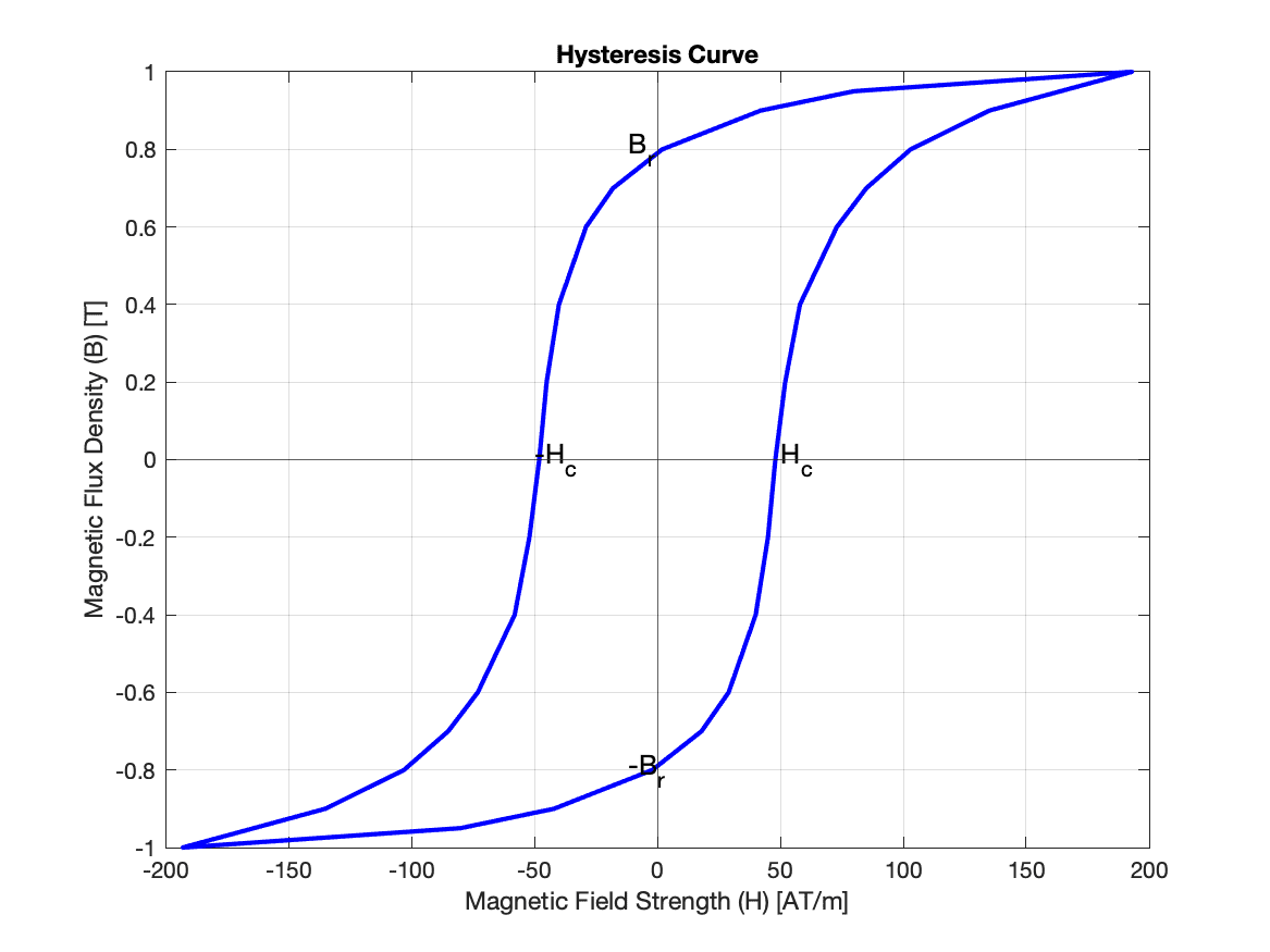
However, the bad news is that, in ferromagnetic materials, the relationship between \( \mathbf{B} \) and \( \mathbf{H} \) is not simply described by a constant \( \mu\) but a variable \( \mu\). Thus, \( \mathbf{B} \) itself depends on the magnetic field. And to make it even more complicated, it also depends on its history. This means that at any point in space, the relationship between \( \mathbf{B} \) and \( \mathbf{H} \) is described by a so-called hysteresis curve (see Figure 2 below).
On one hand, with an increasing field, almost all Weiss domains become oriented and cannot grow anymore, and hence the material is saturated. Further increasing the magnetic field will not lead to a further increase as in vacuum, and the slope of the curve in the fully saturated area is determined by \( \mu_r = 1 \).
On the other hand, after the external magnetic field is removed, some domains still remain oriented, such that some net magnetization remains. This is called remanence, and the resulting magnetic flux density is the remanent flux density \( B_r \) (see again Figure 2 below).
Another important value in the diagram is the coercivity or coercive field strength \( H_c \). It determines the ability of the material to withstand an external magnetic field without becoming demagnetized.
Ferromagnetic materials with high \( H_c \) are called hard magnetic materials. They are used to manufacture permanent magnets. On the other hand, materials with low \( H_c \) are called soft magnetic materials. These are used to guide the magnetic field in transformers, motors, recording heads, magnetic shields, and other applications.
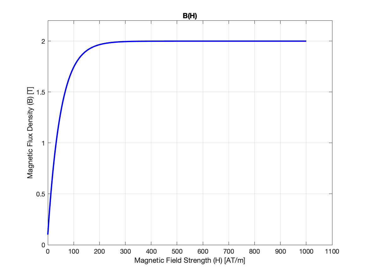
For soft magnetic materials, the hysteresis curve can be simplified to a simple function, represented by the BH-curve, so that the material behavior no longer depends on its history. If it is known in advance that the operating point is in a certain range where the material can be considered linear, a constant \( \mu_r \) is enough to describe the ferromagnetic material. Typical values range from 200 to 10000.
What do you do with a magnetostatic field once you have calculated it? Of course, this depends on the application and the specific problem you want to solve.
Sometimes you are actually interested in the field itself. For example, one often wants to know whether a magnetic core (i.e., the part of a device that is supposed to conduct magnetic flux) has been designed correctly so that it does not go into saturation. Another example is the design of a magnetic shield in cases such as keeping the magnetic field in a certain room or area below certain limits so that measurements or people are not affected.
Most of the time, however, one is not interested in the magnetic field itself but rather in how well an arrangement can store magnetostatic energy (or more general magnetic energy) or maybe how electric coils couple magnetically. This leads to the terms magnetic flux, inductance, or coupling inductance.
Once you have determined the inductances of an arrangement or device, you can use them to characterize it as a lumped element in a circuit-level simulation of an overall system. This is then a form of parameter extraction for a Reduced Order Model (ROM).
Another important application is the calculation of forces or torques resulting from the magnetic field for electrical machines, such as motors, relays, and actuators.
As a branch of electromagnetics that focuses on static magnetic fields, magnetostatics finds numerous important applications in engineering and science. Below are some of the main areas where the study of magnetostatics is highly relevant. It is worth noting that in some of these applications, magnetostatics may not cover all of the electromagnetics design requirements.
Explore Electromagnetics in SimScale
Some examples of Magnetostatics simulations that were conducted using SimScale are presented below:
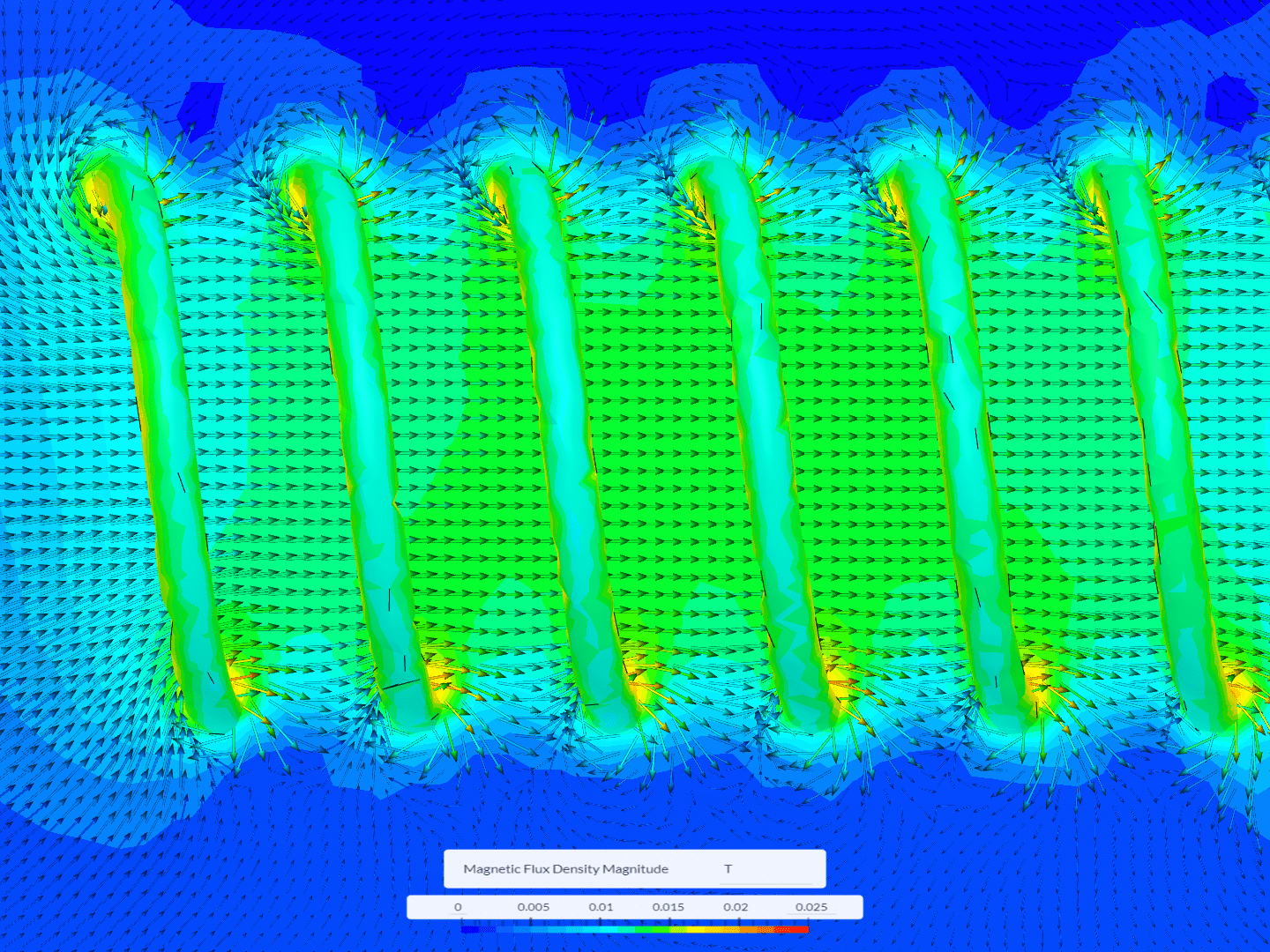
Linear solenoids are electromagnetic devices that generate linear motion, either push or pull, through the action of magnetic fields.
Designers and engineers can optimize the stroke length of linear direct-pushing solenoids by adjusting:
By precisely controlling the magnetic field, they can tailor the solenoid’s stroke to suit specific application requirements, such as in valves, locks, actuators, and other devices where linear motion is essential.
Below is a magnetostatics simulation image illustrating the magnetic field distribution and characteristics of such a solenoid.
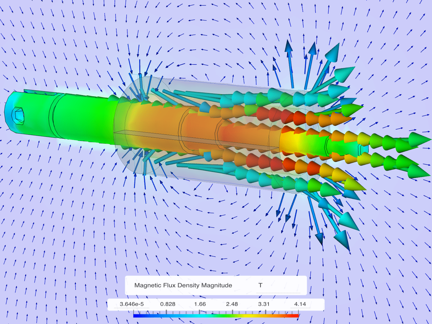
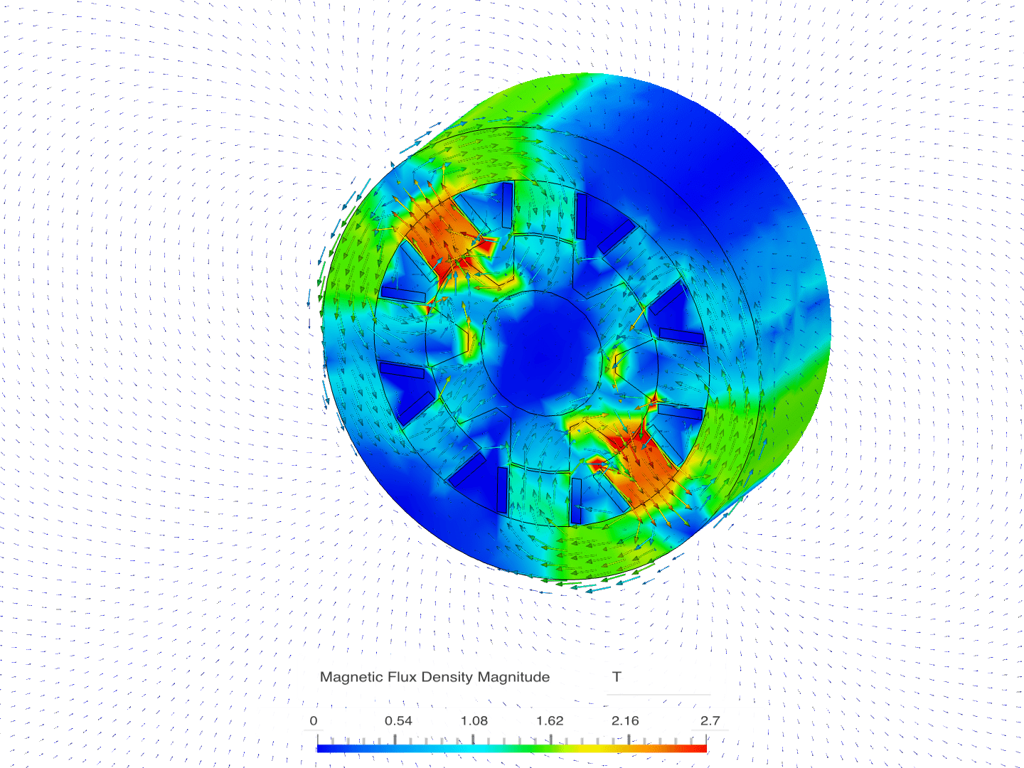
Switched Reluctance Motors (SRMs) are a unique class of electric motors that operate based on the principle of variable magnetic reluctance. Unlike conventional motors that use permanent magnets or electromagnetic fields to generate torque, SRMs utilize the varying reluctance of the magnetic path between the rotor and stator to produce rotational motion.
One of the notable disadvantages of Switched Reluctance Motors (SRMs) is the presence of torque ripple, which results from the abrupt switching of currents during motor operation, leading to vibrations, increased noise, and potential mechanical stresses that may require additional control strategies for mitigation.
Magnetostatics simulations enable a comprehensive understanding of the torque generation mechanisms, torque ripple effects, and efficiency of the motor under different operating conditions. Magnetostatic simulations also aid in optimizing the magnetic circuit, including stator and rotor geometries, magnetic material selection, and winding configurations.
SimScale is a comprehensive multiple physics platform that empowers designers to conduct a wide range of physics simulations within a single project, aiming to streamline the design process and achieve optimized engineering solutions.
Last updated: February 19th, 2026
We appreciate and value your feedback.
What's Next
What is Time-Harmonic Magnetics?Sign up for SimScale
and start simulating now