What is Time-Harmonic Magnetics?
Electromagnetic phenomena are generally described by the Maxwell equations. In the case of linear materials and time-harmonic excitations – i.e., excitations with a sine or cosine time dependence – the electric field, magnetic field, and all currents are also time-harmonic. Time-harmonic magnetics refers to electromagnetic phenomena that vary periodically with time. Then, Maxwell’s equations can be written in a time-harmonic form with angular frequency \(\omega\):
$$\nabla \times \mathbf{H} = \mathbf{J_{free}} + i \omega \mathbf{D}\tag{1a},$$
$$\nabla \times \mathbf{E} = – i \omega \mathbf{B}\tag{1b},$$
$$\nabla \cdot \mathbf{D} = \rho_{free}\tag{1c},$$
$$\nabla \cdot \mathbf{B} = 0\tag{1d}.$$
In this system of equations the electric field \(\mathbf{E}\), the magnetic induction or flux density \(\mathbf{B}\), the dielectric displacement \(\mathbf{D}\), the magnetic field strength \(\mathbf{H}\) and the free current density \(\mathbf{J}_{free}\) are complex vector fields that do not depend on time. The time-dependent electric field, for instance, can be obtained by the relationship \(\mathbf{E}(\mathbf{x},t) = Re ( \mathbf{E}(\mathbf{x}) e^{i \omega t})\). The same applies to the other fields.
These equations will be completed by constitutive equations relating \( \mathbf{B} \) with \( \mathbf{H} \), and \( \mathbf{E} \) with \( \mathbf{D} \) and \( \mathbf{J} \). With the help of these macroscopic laws, detailed bookkeeping of the microscopic charges and currents is no longer necessary. For simple materials, the following applies approximately:
$$ \mathbf{D} = \epsilon \mathbf{E}\tag{2a}$$
$$ \mathbf{B} = \mu \mathbf{H}\tag{2b} $$
$$ \mathbf{J} = \sigma \mathbf{E}\tag{2c}$$
where \(\sigma\) is the electric conductivity, \( \epsilon = \epsilon_{0} \, \epsilon_{r} \) and \( \mu= \mu_{0} \, \mu_{r} \), where with dimensionless constants \(\epsilon_r\) (the relative permittivity) and \(\mu_r\) (the relative permeability) depend on the material. For vacuum and approximately for air, we have \( \mu_{r} = \epsilon_{r} = 1 \). You can read more about Maxwell’s equations in our article on What is Magnetostatics.
Time Harmonic Magnetics (AC Magnetics)
Under certain conditions which are explained in the following section, the term \(i\)\(\omega\)\(\mathbf{D}\), the so-called displacement current, can be omitted from equation (1a). The remaining model becomes:
$$\nabla \times \mathbf{H} = J_{free}\tag{3a}, $$
$$\nabla \times \mathbf{E} = – i \omega \mathbf{B}\tag{3b},$$
completed by Ohm’s Law
$$ \mathbf{J} = \sigma \mathbf{E}\tag{3c},$$
and the relation
$$ \mathbf{B} = \mu \mathbf{H}\tag{3d}. $$
The model above is called the time-harmonic magnetic low-frequency approximation of Maxwell’s equations, sometimes also referred to as magneto-quasistatic approximation, eddy-current model AC magnetics, or simply time-harmonic magnetics.
Note that Equation (1d), which is the divergence of the magnetic flux density, is redundant and not included in the Time-Harmonics model because it is implied by Equation (3b). Consider this: if we take the divergence of equation (3b), then equation (1d) would follow because the divergence of a curl is zero.
The solution of this approximation provides the magnetic field and the induction in the entire computational domain as well as the currents and the electric field in the conductors. If you also want to know the electric field in the non-conductors, which is only the case in very few applications, an additional divergence equation must be solved in the non-conducting region, which provides information about the charges there.
The advantage of the approximation Equation (3) over the full Maxwell equations is that, if done skillfully, it can be solved more easily and quickly.
Scope of Validity
Since all this is an approximation, the following question arises: Under which conditions is this approximation justified? And which applications are correctly described by it? Basically, this is a low-frequency approximation. This means that the model is only valid for sufficiently low frequencies. However, what low enough means depends on the situation; it could be 1 Hz or 1 GHz. Therefore, let’s take a closer look at the validity condition.
It is known that 3 conditions must be fulfilled so that the error made by the approximation is small1.
- The computational domain should be small compared to the wavelength. In other words, the time it takes for the electromagnetic field to propagate through the computational domain should be much shorter than the period of the excitation, so that any change of the excitation can be recognized instantaneously at any place.
- Conductors must have high conductivity, such that \(\omega\) \(\epsilon\) \(\ll\) \(\sigma\), where \(\epsilon\) is the permittivity. This means that charges cannot accumulate in the conductors.
- The geometry should not store any relevant electrical energy, i.e. it does not contain any relevant capacitance.
The first condition means, for example, that antennas and wave propagation cannot be described with it, the last condition implies that resonant circuits and resonance effects are also outside the range of validity.
However, there are many important applications, such as motors, generators, transformers, and many others, that can be described very well with this approximation.
Basically, these are applications in which the magnetic energy change is much more significant than the electrical energy change and induction effects play a role because Equation (3b) is nothing else than the famous Faraday’s law of induction. This means that phenomena such as induced eddy currents, skin and proximity effect are correctly described.
Induced Eddy Currents
Due to the law of induction, a changing magnetic field generates an electric field. If there is a conductor at the location of the electric field, electric currents flow which are self-contained and form vortices. This is why these currents are called eddy currents, and the underlying model is also known as the eddy currents model.
When a conductor, such as a metal plate is subjected to a varying magnetic field, the magnetic flux passing through the conductor changes over time. As a result, according to Faraday’s law of electromagnetic induction, an EMF is induced in the conductor, giving rise to eddy currents.
These currents circulate within the conductor in closed loops, creating localized magnetic fields that oppose the change in the original magnetic field. In general, any factor that leads to variations in the strength or orientation of a magnetic field can give rise to the occurrence of eddy currents within a conductor.
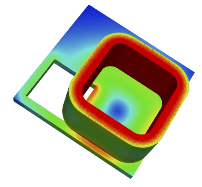
The figure below shows a well-known benchmark model (TEAM 7): a coil above an aluminum plate with a hole in which eddy currents are induced. The benchmark model is used to validate electromagnetic codes.
Skin Effect
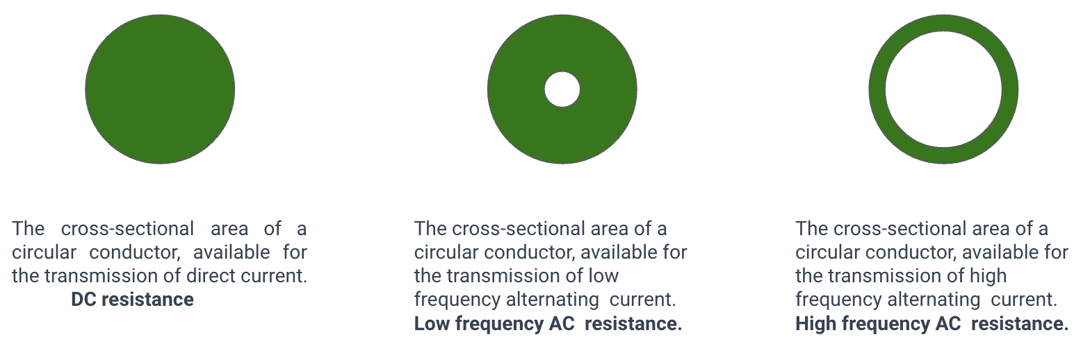
The skin effect is a significant phenomenon in electrical conductors when exposed to alternating current (AC), particularly at higher frequencies. As AC flows through a conductor, the current tends to concentrate near the surface rather than being uniformly distributed throughout the cross-section.
This frequency-dependent behavior results in an increase in the effective resistance of the conductor. At elevated frequencies, most of the current is confined to a thin layer near the surface, leading to a higher resistance compared to direct current (DC) conditions.
The depth to which the current penetrates the conductor is defined as the skin depth, and it is inversely proportional to the square root of the frequency and the conductivity of the material.
As a consequence of the skin effect, an increase in the resistance occurs due to the concentrated current near the surface. This contributes to elevated power losses in the form of heat, making it a crucial consideration in the design of electrical systems, particularly those involving high-frequency AC signals.
Engineers often address this by employing mitigation strategies, such as using hollow conductors or Litz wire with multiple insulated strands, to increase the effective cross-sectional area for current flow.
Proximity Effect
The proximity effect is another important phenomenon in the realm of electrical conductors, especially in situations involving high-frequency alternating current (AC). Unlike the skin effect, which primarily influences the outer layers of a single conductor, the proximity effect is observed in closely spaced parallel conductors carrying AC.
It describes the tendency of the magnetic fields surrounding one conductor to interact with the adjacent conductors, causing a redistribution of current.
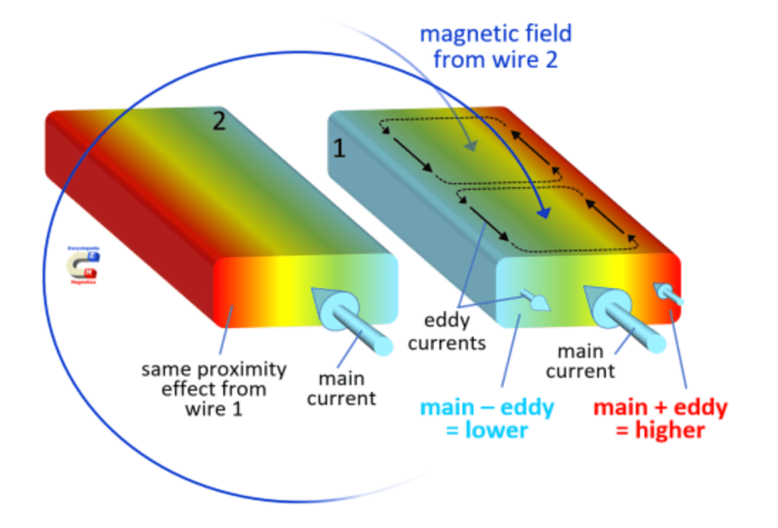
The so-called proximity effect means that the current concentrates with increasing frequency at locations that have the greatest tangential magnetic field strength on the conductor surface. For example, if the two conductors with opposite current directions are close to each other, the magnetic field between the conductors is stronger than on the outer sides, and the current is concentrated on the side facing the other conductor.
At higher frequencies, the alternating magnetic fields generated by the AC in one conductor induce eddy currents in the adjacent conductors. This induces a concentration of current toward the side facing the neighboring conductor, resulting in an uneven distribution of current within each conductor. The proximity effect is most pronounced when the separation between conductors is comparable to or smaller than the skin depth.
Similar to the skin effect, the proximity effect increases effective resistance, contributing to higher power losses in the system. Mitigation strategies are employed to address these effects, such as adjusting the spacing between conductors or using specific geometric configurations to minimize the impact. Furthermore, the proximity effect is a critical consideration in the design of high-power transmission lines and closely bundled cables.
Applications of Time-Harmonic Magnetics
Here are several examples of applications that can be correctly modeled by time-harmonic magnetics. You may also refer to “What is Electromagnetic Induction” for further examples.
Transformers
Transformers are indispensable devices in the realm of electrical engineering, serving as key components in power transmission and distribution systems.
Operating on the principle of electromagnetic induction, transformers facilitate the efficient transfer of electrical energy between two or more circuits. By transforming voltage levels, transformers enable the long-distance transmission of electricity, contributing significantly to the functionality of power grids.
Consisting of a core made of ferromagnetic material and primary and secondary winding coils, transformers manipulate magnetic fields to induce voltage across their windings. This process allows for the step-up or step-down of voltage levels, catering to the diverse needs of power distribution networks.
Transformers come in various types and sizes, ranging from small, household transformers to large, utility-scale units, each designed to meet specific demands within the intricate web of electrical infrastructure.
Time-harmonic simulation proves invaluable in optimizing the core material, winding configuration, predicting magnetic field distributions, losses, and temperature variations (when coupled with a thermal solver – to be expected on SimScale soon), offering insights that contribute to the development of efficient and reliable transformer designs within the dynamic landscape of electrical power systems.
Non-Destructive Testing (NDT)
Non-destructive testing (NDT) encompasses techniques crucial for evaluating material integrity without causing damage. Two significant methods based on low-frequency magnetic approximation are Alternating Current Field Measurement (ACFM) and eddy-current testing.
ACFM involves inducing an alternating magnetic field into ferromagnetic materials, detecting surface and near-surface flaws through the analysis of magnetic flux leakage. This technique is highly sensitive and commonly employed in industries such as oil and gas, aerospace, and manufacturing for inspecting critical components like pipelines and welds.
Eddy-current testing, on the other hand, utilizes electromagnetic induction to assess conductive materials. By inducing eddy currents through an alternating current, disruptions caused by defects, such as cracks or changes in conductivity, are detected and analyzed.
Eddy-current testing is widely used in aerospace, automotive, and manufacturing industries for its ability to identify surface and subsurface flaws, providing valuable insights into material integrity without causing damage.
Both ACFM and eddy-current testing play pivotal roles in ensuring the quality and reliability of critical structures and components across various applications.
Skin Effect in Bus Bars
In the context of busbars, the phenomenon known as the skin effect plays a crucial role in the distribution of alternating current (AC). As previously discussed, the skin effect leads to a non-uniform current distribution, concentrating the flow towards the surface of the conductor.
The higher the frequency of the AC, the more pronounced this effect becomes. Engineers must attentively account for skin effect when designing busbars, as it influences the effective cross-sectional area for current flow and necessitates optimization of dimensions to ensure optimal performance, especially in scenarios with elevated frequencies.
Induction Heating
Induction heating is a method of generating heat in conductive materials through electromagnetic induction. This process relies on the principle of electromagnetic fields inducing electric currents within a target material, typically a metal. An alternating current passes through a coil, creating a rapidly changing magnetic field. When a conductive material is placed within this field, eddy currents are induced within the material, resulting in resistive heating due to its electrical resistance. Induction heating can be highly precise and allows for localized and controlled heating without direct contact with the heat source.
Time-Harmonic Magnetics in SimScale
SimScale is a comprehensive multiple physics platform that empowers designers to conduct a wide range of physics simulations within a single project, aiming to streamline the design process and achieve optimized engineering solutions. SimScale’s latest physics release has been electromagnetics, currently covering low-frequency electromagnetics. With its magnetostatics simulation and the long-awaited time-harmonic magnetics simulation tool, SimScale allows engineers and designers to run various electromagnetics simulation runs simultaneously.
Explore Electromagnetics in SimScale
This can also be run in parallel with other analysis types, all in one, easy-to-use online workbench, allowing for comprehensive analysis of multiple physics at the same time without being hindered by hardware limitations or software installations.
References
- https://www.researchgate.net/publication/3113218_Estimating_the_Eddy-Current_Modeling_Error
- https://www.e-magnetica.pl/doku.php/file/proximity_effect_proximity_loss_magnetica_png
Last updated: February 19th, 2026
Did this article solve your issue?
How can we do better?
We appreciate and value your feedback.
What's Next
What is Electromagnetic Induction?

