Documentation
In Pedestrian Wind Comfort analysis, the Simulation control feature allows you to control the following parameters:
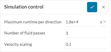
This is the time value in seconds which decides the maximum physical time for which the Pedestrian Wind Comfort simulation will run for each wind direction. Hence, if four wind directions are being simulated then the actual physical time the simulation run would take is four times this value. The simulation run is automatically canceled if this value is exceeded.
It is important to assign enough time for simulation to finish, but it shouldn’t be unexpectedly long causing you to end up burning a huge amount of core hours.
So how can you know the minimum time required to complete the simulation?
There is no direct way of knowing that. But the concept of “number of fluid passes” can be helpful to get an overall idea.
Using the number of fluid passes, the user can decide the length of the transient simulation. This is helpful because all PWC simulations are based on the lattice-Boltzmann method, which is inherently transient and, therefore, time-dependent.
Typically we say that the first ‘fluid pass’ is required for the simulation to become ‘steady’, i.e., we expect any radical results due to the initial conditions to be washed out of the domain. We usually leave another ‘fluid pass’ for the simulation to become somewhat periodic and any results in the third pass are fair to be used as ‘results’. Average results are obtained in the final 20% of the simulation and by default 3 fluid passes is the assigned value.
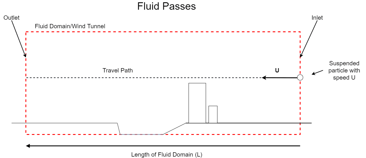
The best way to imagine a fluid pass is that some suspended smoke particle enters the inlet and leaves in a straight line through the outlet. Considering the domain length, and the velocity (reference velocity is usually 10 \(m/s\)) then:
$$N \times \frac{L}{U}=t$$
Where \(L\) is the domain length, \(U\) is the velocity, and \(N\) is the number of fluid passes and \(t\) is the transient simulation time.
Therefore, if a domain was 1 \(km\) long and a reference velocity of 10 \(m/s\) was used a fluid pass would be 100 \(s\), and consequently 3 fluid passes would be 300 \(s\). In conclusion, the number of fluid passes defines the simulation time.
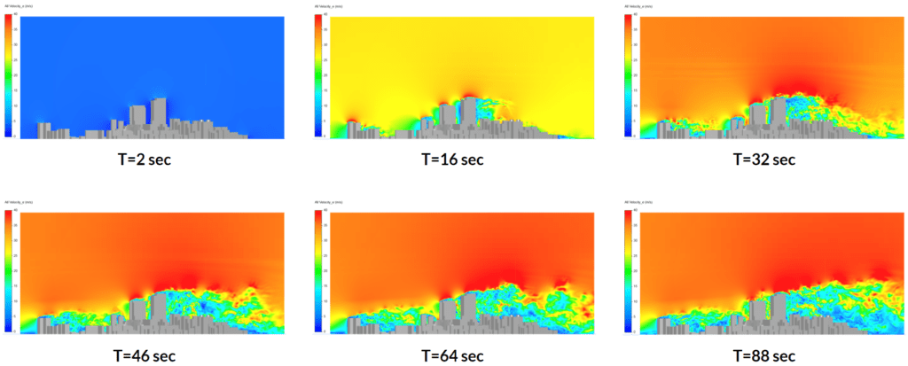
Figure 3 clearly shows the transient behavior of the flow. During the initial phase (up to 32 seconds), the flow is being developed. Later on, we do not see much change in the flow field, which means that the flow field reached a steady-state. Usually, using at least 3 fluid passes is convenient to extract useful results.
This feature is available for both PWC and Incompressible LBM simulations. Like any explicit numerical method, Lattice Boltzmann’s methods can only solve a transient solution if the time step is reasonably set. If a timestep becomes too long, it will have numerical issues causing the simulation to finish prematurely, with an error and without returning results.
It’s important to note that velocity scaling, in this sense, does not impact the results. It’s not the same as Reynolds scaling and only impacts the simulation stability. The wind speed results at the end of the simulation will not be different, nor is the Reynolds number affected, and similarities should be drawn to the Courant number in other CFD codes.
Our default simulation setup makes this very rare, and for a vast majority of LBM/PWC users, this documentation page will be irrelevant. However, for the few who have cases that struggle, this documentation will help you.
Uniquely In LBM, the maximum stability parameter can be defined by the inverse of the ratio of specific heats. For air, this is approximately 0.7. However, we should not be near this value for incompressible solvers. Instead, we should not exceed 0.3.
Furthermore, because the compressibility is 0.3 globally, doesn’t mean that local speeds are not higher, and therefore, compressibility also increases. In fact, it makes sense to use a range of values between 0.01 and 0.25, where the default stability parameter is 0.1 which makes the simulation experience robust.
Warning
The stability parameter affects the time step size linearly. For example, a simulation run for 100 seconds, with a stability parameter of 0.1, might have a time step size of 1 second, meaning that we need to solve 100-time steps. In contrast, dropping the stability parameter to 0.05 and the timestep also drops to 0.5 seconds, and we then need to solve 200-time steps to complete 100 seconds of simulated time.
Last updated: July 6th, 2023
We appreciate and value your feedback.
What's Next
Simulation Control for Wind Comfortpart of: Pedestrian Wind Comfort Analysis
Sign up for SimScale
and start simulating now


