Supersonic Shock Tube

This validation case demonstrates the accuracy of the ‘Multi-Purpose’ solver in SimScale for a compressible shock tube problem. The case is based on Sod’s classic Riemann problem¹ , which produces three distinct wave structures: a rarefaction fan, a contact discontinuity, and a shock wave, occurring after the removal of a diaphragm separating two regions of gas at different pressures. SimScale results are compared against the exact analytical solution for an ideal gas.

Problem Description

A one-dimensional tube is divided at its midpoint by a diaphragm. Gas on the left side is at a higher pressure and density than gas on the right side. When the diaphragm is instantaneously removed, three wave structures propagate outward:

A rarefaction wave propagating to the left, expanding the high-pressure gas.
A contact discontinuity propagating to the right, across which density and temperature are discontinuous, while pressure and velocity remain continuous.
A shock wave propagating to the right, compressing the low-pressure gas.

Because the exact solution to this Riemann problem is known analytically for an ideal gas, the case serves as a rigorous benchmark for compressible solvers. It verifies that the solver correctly captures shock speed, wave positions, and the distribution of primitive variables across all three wave regions.

View Project

Geometry and Initial Conditions

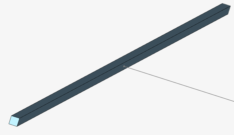
The domain is a straight tube of unit length. The diaphragm is located at the midpoint (\(x = 0.5\) \(m\)). While the implementation of this problem in CFD is typically performed in 2D, SimScale uses 3D models. To address computational cost, the model dimensions were adjusted in width and height to allow for 5000 cells along the 1 \(m\) channel length while ensuring only a single element along the thickness and height. Initial conditions are applied as two uniform states on either side:

Shock Tube CFD — Figure 1: CFD domain with the dimensions of 0.0002 x 0.0002 x 1 \(m\).

Parameter	Left side (high pressure)	Right state (low pressure)
Pressure	5.0 × 10⁵ \(Pa\)	2.0 × 10⁴ \(Pa\)
Temperature	303 \(K\)	303 \(K\)
Velocity	0 \(m/s\)	0 \(m/s\)

The fluid is treated as an ideal gas with a specific heat ratio \(\gamma = 1.4\) and gas constant \(R = 287\) \(J/(kg·K)\). Results are evaluated at \(t = 4.0 × 10^{-4}\) \(s\) after diaphragm removal.

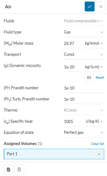
The fluid employed in the Sod Shock Tube Problem is air, modeled as an ideal gas, under the assumptions of zero viscosity and negligible thermal conductivity \(Pr = 1.0 × 10^{-10}\).

Supersonic Shock Material — Figure 2: Air properties for supersonic shock simulation.

Simulation Setup

Setting	Value
Analysis type	‘Multi-Purpose’
Fluid model	Ideal gas
Specific heat ratio (\(\gamma\))	1.4
Domain length	1.0 \(m\)
Diaphragm position	\(x = 0.5\) \(m\)
Simulation end time	4.0 × 10⁻⁴ \(s\)

Initial conditions for pressure, density, and velocity were applied as two-region field initializations on either side of the diaphragm position using the ‘Initial conditions’ settings in the simulation tree.

Note

This case requires pressure and temperature initial conditions, which are available in the ‘Multi-Purpose’ analysis type. The ability to specify non-uniform initial conditions across regions of the domain is essential for reproducing the shock tube setup correctly.

Results

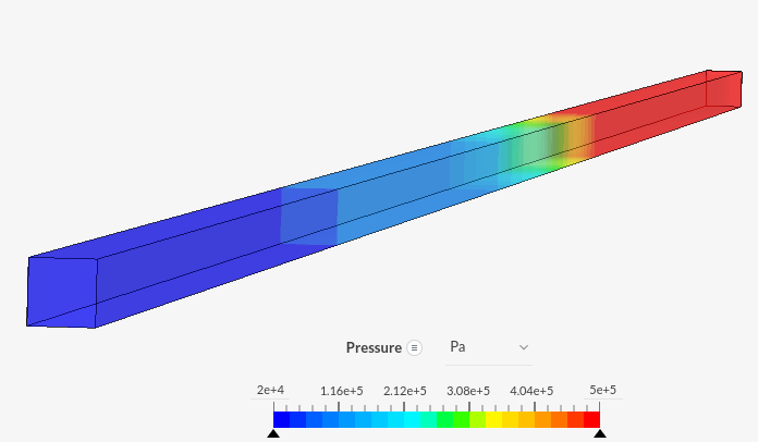
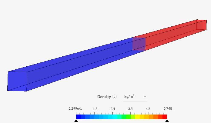
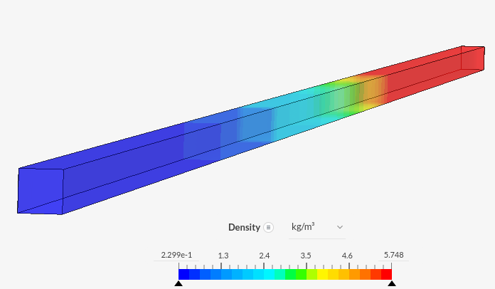
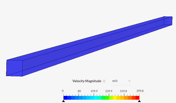
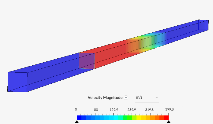
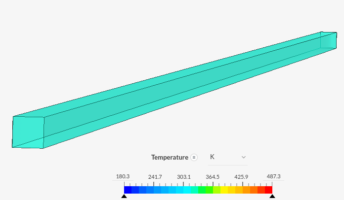
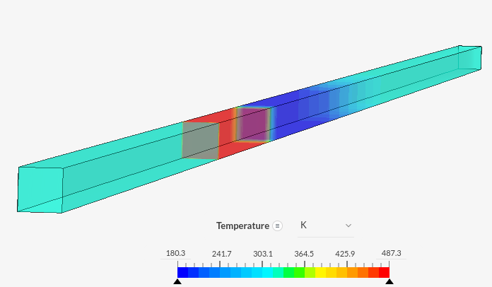
The plots below compare the SimScale ‘Multi-Purpose’ solver results against the exact analytical solution at \(t = 4.0 × 10^{-4}\) \(s\). Four primitive variables are compared along the tube axis: pressure, density, and velocity.

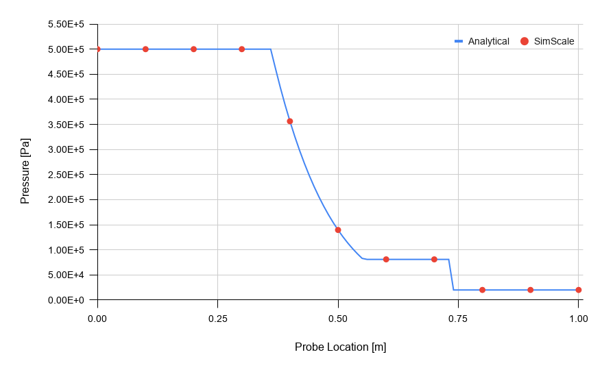
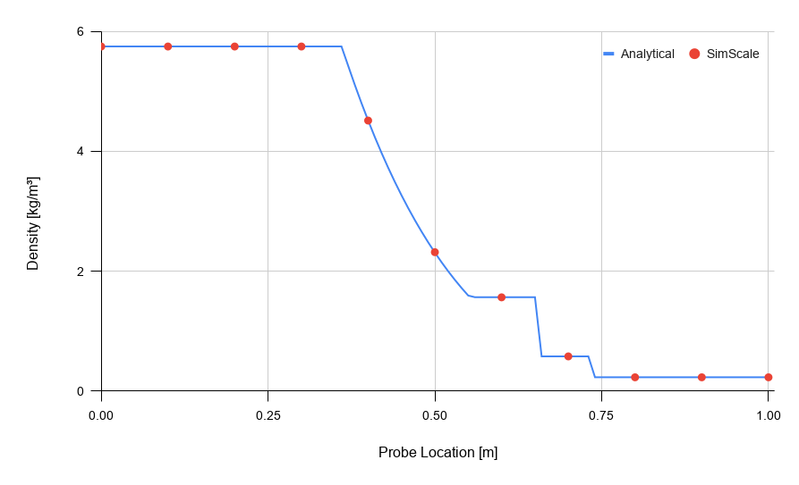
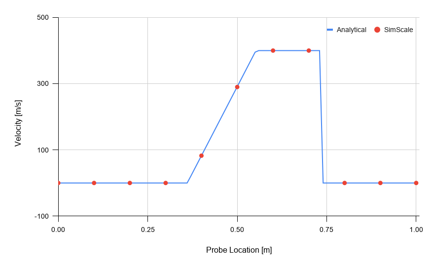
Figure 4: Comparison between the analytical and SimScale results for Density.

Figure 5: Comparison between the analytical and SimScale results for Velocity.

The solver correctly captures the position and shape of all three wave structures. Key observations from the comparison include:

The shock wave position and the post-shock pressure and density match the analytical values with high accuracy.
The contact discontinuity position is reproduced accurately, and the density jump across it is well-resolved.
The rarefaction profile follows the expected smooth expansion and agrees closely with the analytical curve across the domain.

Transient Contours

The table below summarizes the shock behavior at \(t = 4.0 × 10^{-4}\) \(s\), comparing the phenomena with the initial state.

Conclusion

The SimScale ‘Multi-Purpose’ solver reproduces the Sod shock tube solution with high accuracy for an ideal gas. The positions and magnitudes of the shock wave, contact discontinuity, and rarefaction fan are all in close agreement with the analytical Riemann solution. This confirms that the solver correctly handles the propagation of compressible wave structures and the associated discontinuities in density, pressure, and velocity that arise in supersonic and transonic flow regimes.

References