Validation case: Conjugate Heat Transfer in a Battery Pack

The aim of this project is to demonstrate the validity of SimScale’s CHT v2.0 and CHT IBM solver by performing a conjugate heat transfer analysis of a battery pack and comparing the following parameter:

•  Local temperatures at available thermocouple locations

The simulation results of SimScale were compared to the results presented in [1]. Code Verification is also carried out by comparing the SimScale results to Fluent results.

Geometry

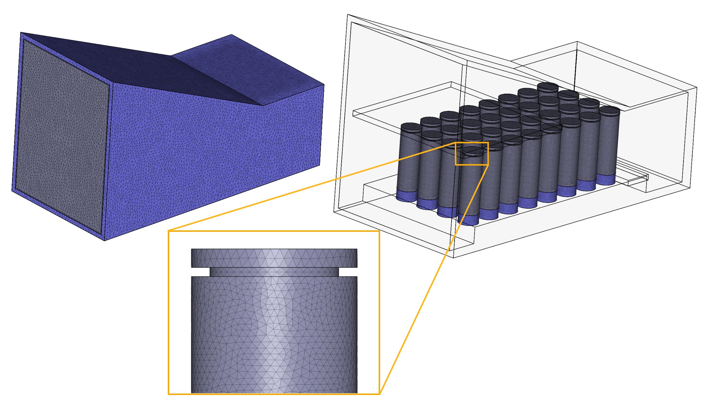
The geometry can be seen below:

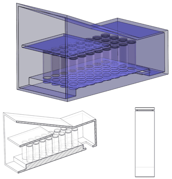
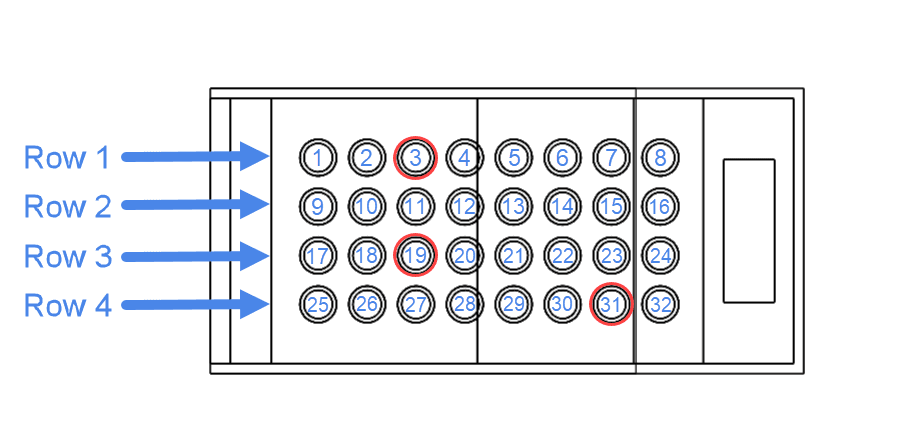
It represents a 1:1 model reverse-engineered from images in the publication. The battery pack consists of 32 (8×4) cell configuration.
The thermocouple location on the leeward side of the cells has been used for validating the conjugate heat transfer solver:

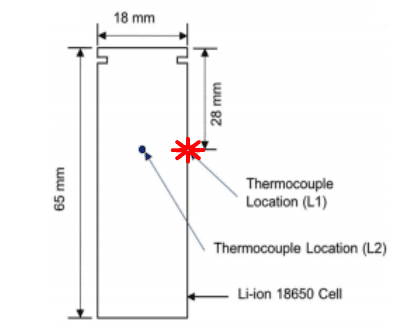
The thermocouple readings from cells 3, 19 and 31 have been used for the comparison:

Analysis Type and Mesh

Tool Type: OpenFOAMⓇ

Analysis Type: Compressible, steady-state analysis with the CHT v2.0 and CHT IBM solver.

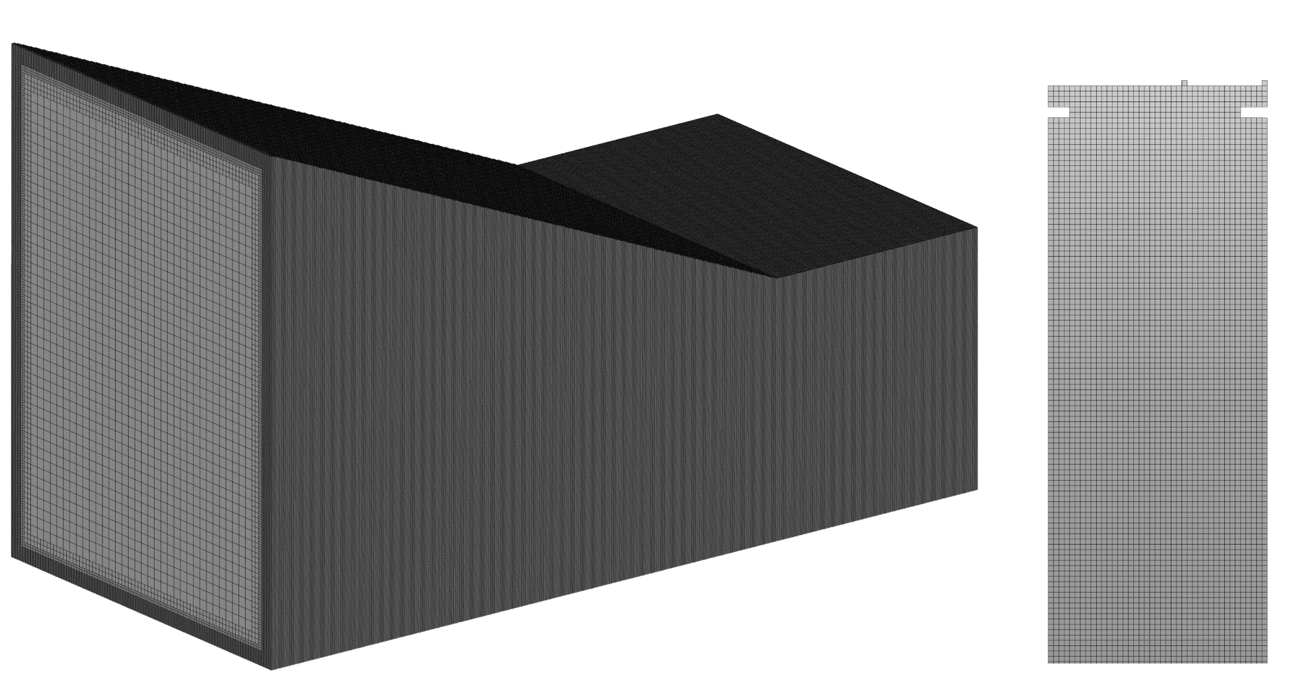
Mesh and Element Types:

The Standard mesher algorithm with tetrahedral and hexahedral cells was used to generate the mesh. A mesh sensitivity analysis has been carried out to determine the dependence of the CHTv2 solver temperature predictions on the mesh, while using lead as the material of the cells:

Mesh Type	Number of cells/nodes	Temperature@L1-cell3 [\(°C\)]	Temperature@L1-cell19 \([°C]\)	Temperature@L1-cell31 \([°C]\)
Mesh 1	3.6M cells, 1.1M nodes	29.535	31.065	26.816
Mesh 2	11.2M cells, 3.5M nodes	30.794	31.114	27.218
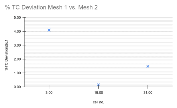
%TC deviation (Mesh 2 – Mesh 1)		4.089	0.157	1.477

Maximum temperature deviation of 1.2 \(°C\) (~4.1%) between Mesh 1 and Mesh 2, was observed at leeward side of cell 3. In the following figure the percentage of temperature deviation in degrees Celsius (% TC) at measurement location L1 is displayed for three different mesh configurations as well:

In order to estimate the physical properties of the cells, a material sensitivity study has also been carried out, using three different materials:

• Lead (low conductivity)
• Aluminium (medium conductivity)
• Copper (high conductivity)

Comparing L1 temperatures for the three materials, according to the diagrams below, aluminium cells show the closest match:

• to thermocouple readings at all three measurement cells (3,19 and 31);
• to ANSYS Fluent predictions at all three measurement cells (3,19 and 31). 

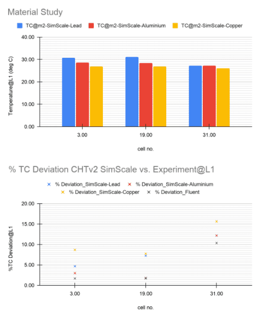
Hence, based on the material and mesh sensitivity analyses, aluminum cells and “Mesh 2” have been used for the final validation using CHT v2.0 analysis.

For CHT IBM analysis the IBM solver creates a Cartesian mesh that does not resolve every part separately as in a body-fitted meshing approach, but refines the Cartesian grid towards geometrical and topological details and immerses the geometry into it. The detailed treatment is done on the solver level instead.

Simulation Setup

Fluid Material:

• Air
  • Dynamic viscosity \((\mu)\) = 1.83e-5 \(m^2 \over\ s\)
  • Specific heat = 1004 \(J \over\ (kg \times\ K)\)

Solid Materials:

• Wood
  • Isotropic
  • Thermal conductivity \((k)\) = 0.16 \(W \over\ (m \times\ K)\)
  • Specific heat = 1260 \(J \over\ (kg \times\ K)\)
  • Density \((\rho)\) = 500 \(kg \over\ m^3\)
• Aluminum
  • Isotropic
  • Thermal conductivity \((k)\) = 235 \(W \over\ (m \times\ K)\)
  • Specific heat = 897 \(J \over\ (kg \times\ K)\)
  • Density \((\rho)\) = 2700 \(kg \over\ m^3\)

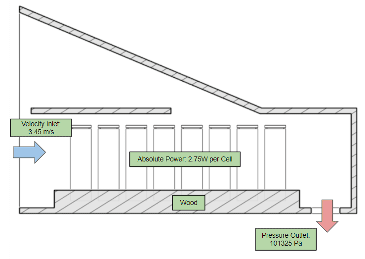
Boundary Conditions:

• Room temperature, \((T)\) = 23 \(°C\)
• Inlet velocity = 3.45 \(m \over\ s\)
• Outlet pressure = 101325 \(Pa\) (fixed value)
• Absolute power = 2.75 \(W\) per cell 
• No-slip walls

Result Comparison

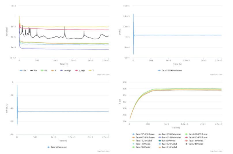
Convergence below 1e-3 has been achieved. Calculated physical quantities such as inlet pressure, outlet velocity, and cell average temperatures have also been allowed to converge to stable values:

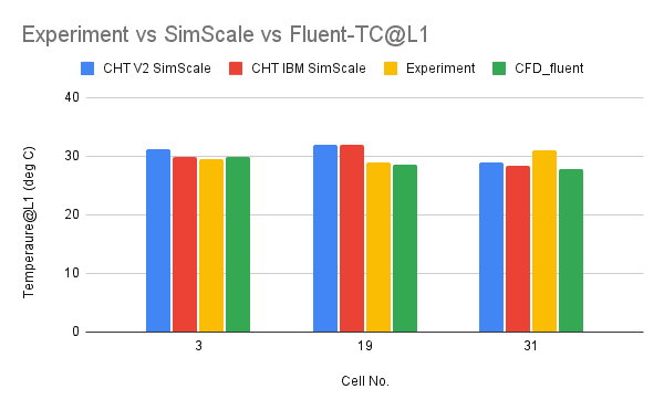
The final temperature values are displayed in the following table:

Cell No.	CHT V2 SimScale\([°C]\)	CHT IBM SimScale\([°C]\)	Experiment \([°C]\)	CFD_fluent \([°C]\)
3	31.22	29.42	29.42	29.92
19	32	31.86	29.01	28.52
31	28.85	28.45	30.99	27.78

Comparing CHTv2 solver predictions to thermocouple readings@L1, temperature deviations of:

• Cell 3: 0.53 \(°C\) (1.8%)
• Cell 19: 2.85 \(°C\) (9.8%)
• Cell 31:  2.54 \(°C\) (8.2%)

The temperature deviations predicted from the CHTv2 solver are in good comparison with ANSYS Fluent and the experimental data.

There are some minor deviations and the reasons could be:

1. The orientation of the battery arrangement within the battery pack has been misrepresented in the publication (experimental setup);
2. The battery material has been approximated via a sensitivity study.

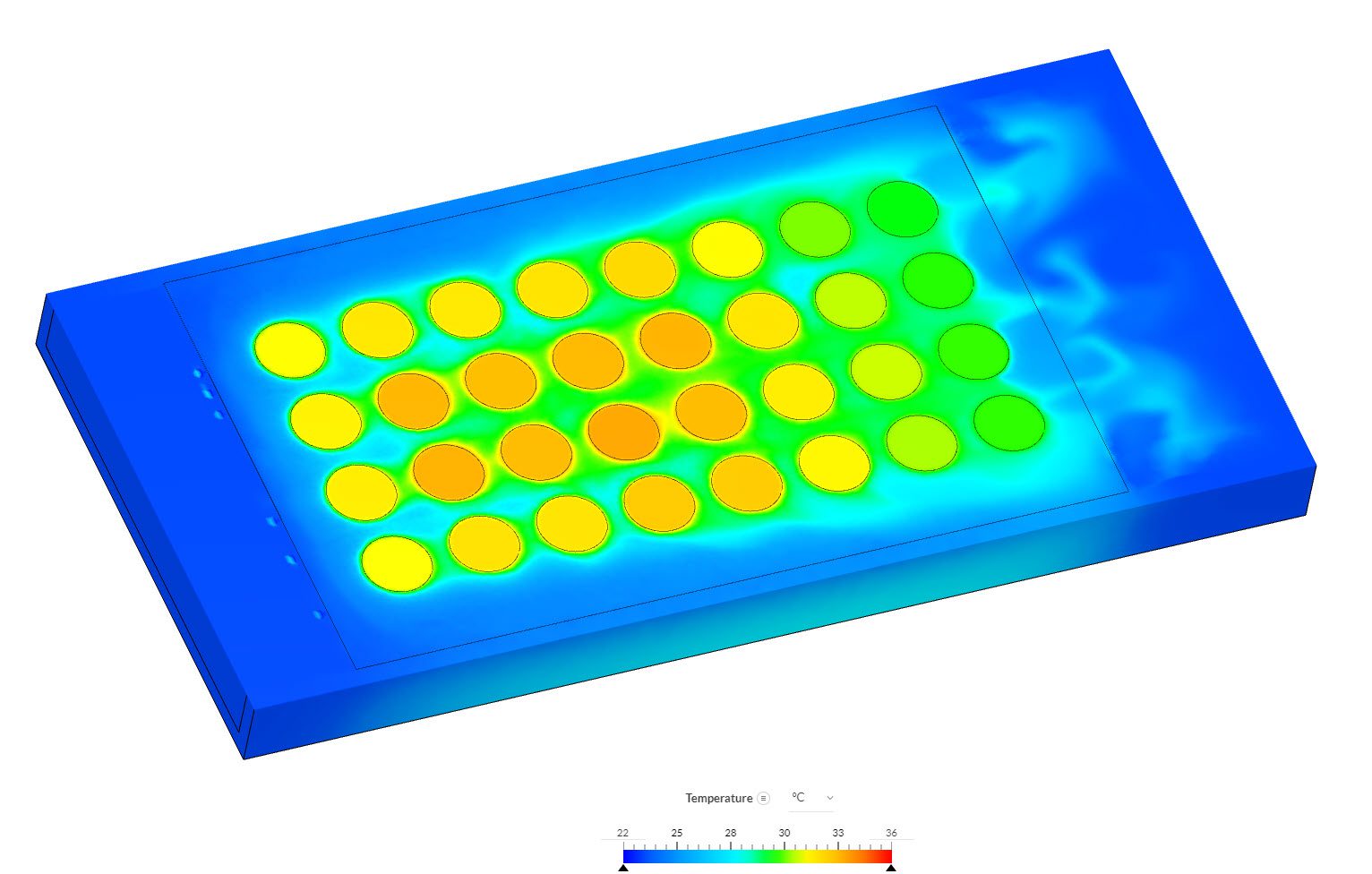
In the following image, the temperature distribution across the flow domain indicates the heat transfer from cells to the air inside the battery pack. The cutting plane displayed is normal to the z axis:

Last updated: April 9th, 2024