Thermal Management Tutorial: CHT Analysis of an Electronics Box
This advanced thermal management tutorial describes the setup and analysis of the cooling of an electronics box. The scenario consists of a box with several components, being cooled down by a fan.
All electronic devices generate heat during their operation. Components and materials used in these devices have individual maximum temperature limitations. Therefore, thermal management is crucial for system reliability and preventing failure.
Simulation is a cost-efficient method to test different cooling strategies and optimize your solution. This is a great advantage to prevent time-consuming and expensive prototyping and physical testing procedure.
This tutorial teaches you how to:
- Select suitable boundary conditions for thermal management/electronics cooling
- Assign materials for different components
- Define individual contact properties
- Judge the calculation stability
We are following the SimScale workflow:
- Prepare the CAD model for the simulation
- Set up the simulation
- Create the mesh
- Run the simulation and analyze the results
1. Prepare the CAD Model and Select the Analysis Type
Import the tutorial project into your Workbench by clicking the button below:
Clicking this link leads to the following view:
1.1 Editing the CAD
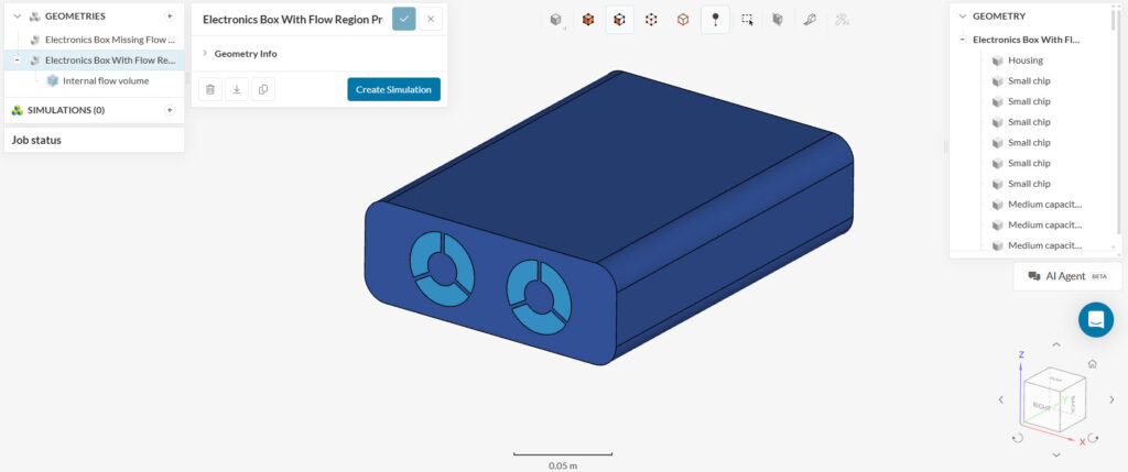
The simulation project contains two geometries. The first one, named Electronics Box Missing Flow Region still needs a final CAD preparation step before it can be used in a simulation. For interested readers, the flow volume extraction step will be explored below.
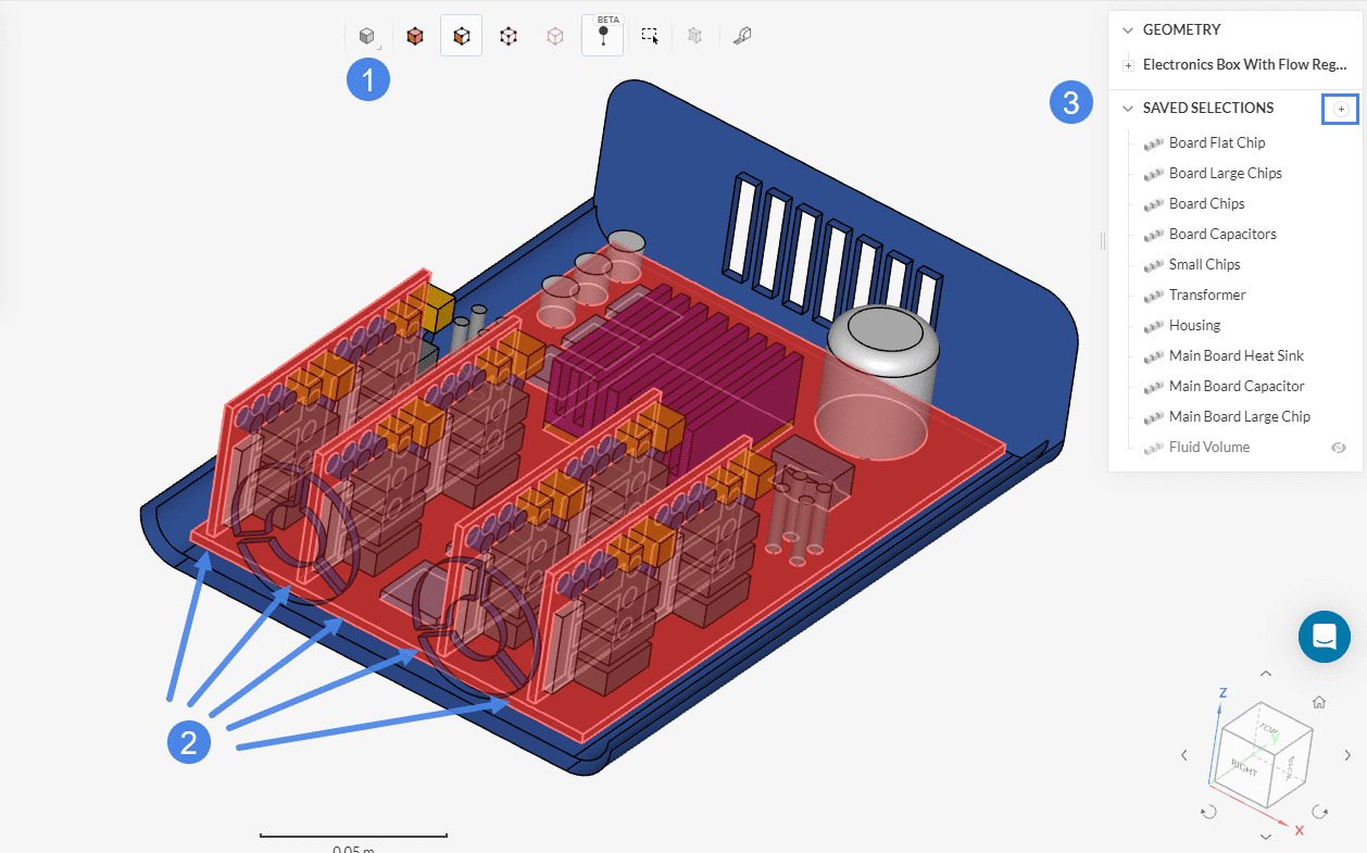
The second geometry will be the one used in this tutorial. Besides the flow region that is already available in it, the second geometry also contains a series of pre-defined Saved Selections that will be used throughout the tutorial. If you are not interested in the flow volume extraction workflow, please skip the note below.
Generating an Internal Fluid Volume
For every internal fluid simulation, we need a volume in the CAD model representing the fluid domain. In order to create a flow region or make modifications to the CAD model, we are going to use the CAD environment. To modify a CAD model, simply select the geometry from the list—the available CAD operations will then appear in the top toolbar. You can either work directly on the original model or create a duplicate and apply your changes to the copy.:
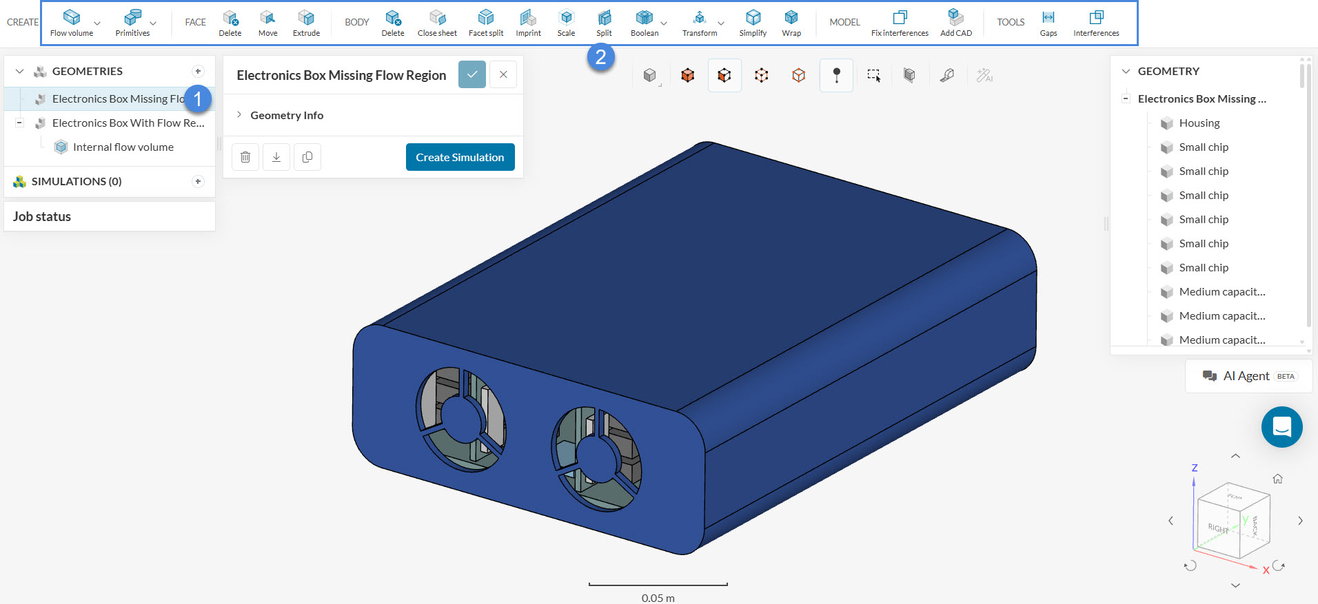
After selecting the first geometry, the geometry operations will appear at the top. The interface looks as follows:

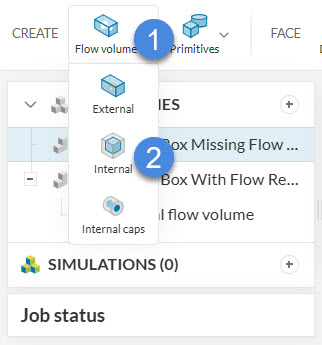
Next, create an internal flow volume operation by hovering over the ‘Flow Volume’ icon and selecting ‘Internal’.
To create the internal fluid volume, select a face of the housing that will be adjacent to the boundary face. This will define a starting point (source) for the internal fluid volume creation and is referred to as a seed face.
Since the housing of the electronic box has two open faces, we have to define two boundaries, which will limit the creation of the internal fluid volume. For the electronic box, select the front and the backside of the housing, as the boundaries.
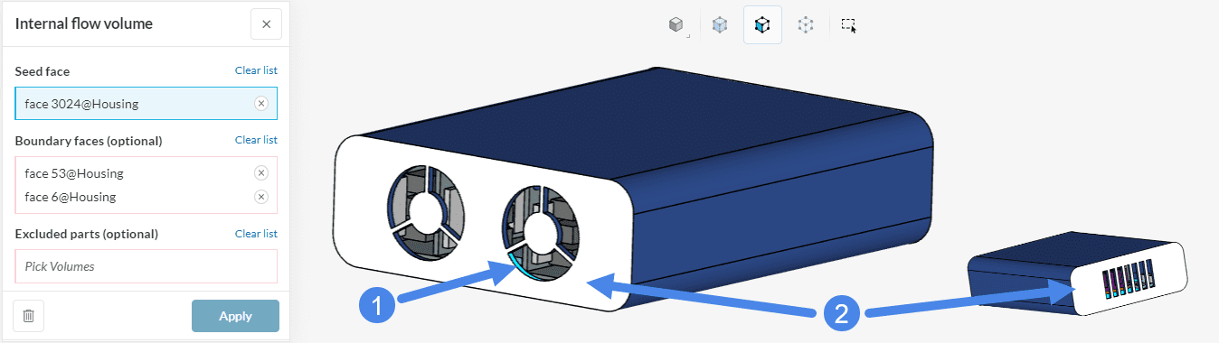
- Select a seed face inside adjacent to the boundary face.
- Select the boundary faces for the internal fluid volume.
- Hit ‘Apply’.
Now all modifications should be saved to the selected CAD model, and you can proceed to simulation setup directly.
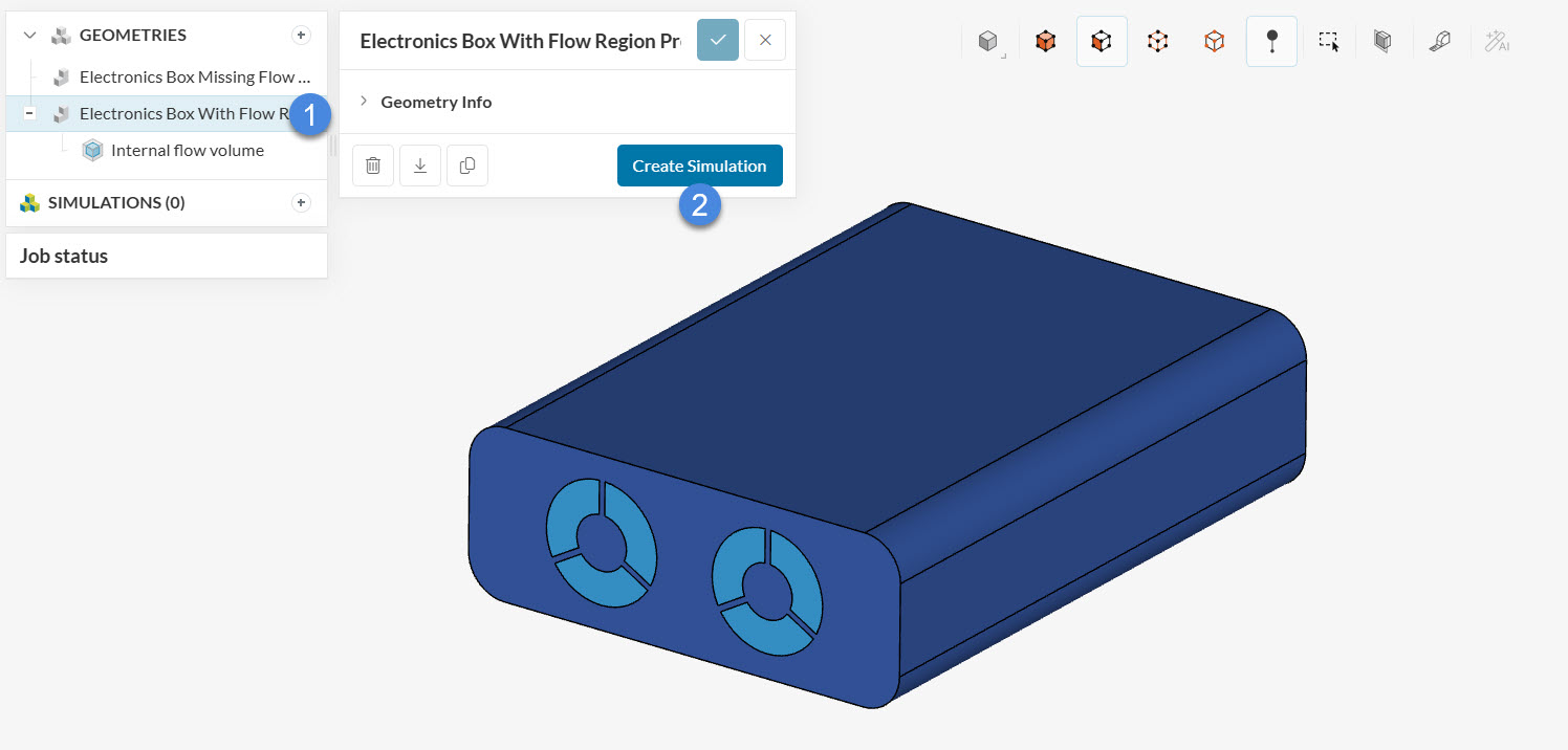
For this simulation, use the ‘Electronics Box Flow Region Prepared’ geometry, where only the saved selection for the boards is missing.
1.2 Saved Selections for the Boards
To continue with the simulation setup, select the ‘Electronics Box Flow Region Prepared’ geometry. To create the sets for the boards, switch to the volume selection mode, expand the geometry parts list, and select the following parts: ‘Board 4’, ‘Board 3’, ‘Board 2’, ‘Board 1’, and ‘Main Board’.
After selecting the parts click on the plus icon next to Saved Selections and name the selection ‘Boards’.
2. Simulation Setup
2.1 Create a Simulation
Once all saved selections are ready, select the ‘Electronics Box Flow Region Prepared’ geometry and click on the ‘Create Simulation’ button as presented in the following picture:
Now the analysis selection widget will pop up:
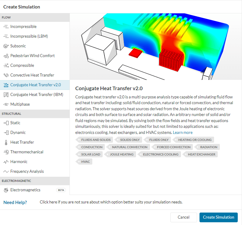
Within the analysis type widget, all analysis types available in SimScale are listed. Selecting one of them shows a description of them. For this thermal management simulation, we will use the ‘Conjugate Heat Transfer’ option. Afterward, hit the ‘Create Simulation’ button to confirm the selection.
Did you know?
The analysis type you choose within the simulation library depends on the physics that need to be accounted for, the results that you are interested in, and what parameters you have.
- In this simulation, we want to see the heat transfer both within the solid parts as well as from the solids to a fluid. Hence we need to select the Conjugate Heat Transfer analysis type.
- If you are only interested in the heat transfer within solids, you can simplify the simulation process by performing a Heat Transfer analysis.
- On the other hand, assuming you are only interested in the heat transfer within a fluid, you would go for Convective Heat Transfer.
2.2 Global Settings
Now you have successfully created a CHT simulation. On the left-side panel, you should see a simulation tree named Conjugate heat transfer, as shown in the picture below:
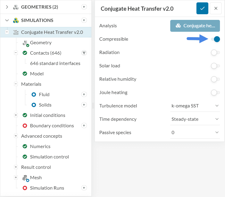
Take this opportunity to access the global simulation settings and toggle on the Compressible option. For electronics cooling applications, the temperature gradients experienced by the fluid are often large, so compressible effects are of interest.
In the global settings, we can also decide whether or not we want to take into account radiation. For this tutorial, radiation will remain toggled off.
Did you know?
The k-omega SST turbulence model switches between the k-omega and k-epsilon model automatically, therefore it takes the advantage of both models and can be used for the majority of turbulent flow simulations.
Have a look at
this page to learn more about the global simulation settings.
2.3 Geometry
The next entry in the simulation tree is Geometry. Since we are already using the geometry of interest, we can skip this tab entirely.
2.4 Contacts
A thermal interface is a commonly used feature when it comes to electronics cooling and thermal management applications. In SimScale, Contacts between parts are detected automatically as soon as a new CHT simulation is created. In the geometry used for this tutorial, you should see a total of 646 standard interfaces.
By default, all contacts will be Coupled, which means that heat can flow through the interfaces without any thermal resistance. Depending on the physics of your design, you might be interested in applying a certain resistance to contacts of interest. The sections below explore this workflow.
Changing The Thermal Conductivity Of The Large Chip and Conductor
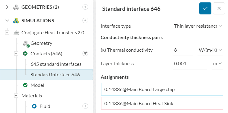
For this analysis, we want to simulate a 0.001 \(m\) thermal paste with 8 \( \frac{W}{mK}\) thermal conductivity between the large chip and heat sink. The image below describes the workflow:
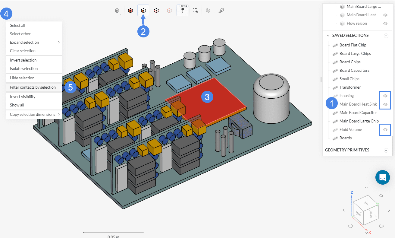
- In the Saved Selections tab, click on the ‘eye’ icon next to Housing, Main Board Heat Sink, and Fluid Volume to hide them.
- Make sure that face selection is enabled.
- Click on the top face of the large chip to select it.
- Right-click on the viewer.
- Select ‘Filter contacts by selection’.
Now the contact definition for the interface of interest is shown. Adjust the Interface type to ‘Thin layer resistance’ with a Thermal conductivity of ‘8’ \( \frac{W}{m K} \) and a Layer thickness of ‘0.001’ \(m\):
Important Note
Avoid adding thin layered materials (thermal paste, insulator on winding, etc.). Including these materials in the model increases the mesh density and the computational expense. Instead, you can define them as a Contact interface as described earlier in this section.
2.5 Model
Under the Model tab, the user can define the gravity magnitude and direction. Please note that the definition is based on the global coordinate system:
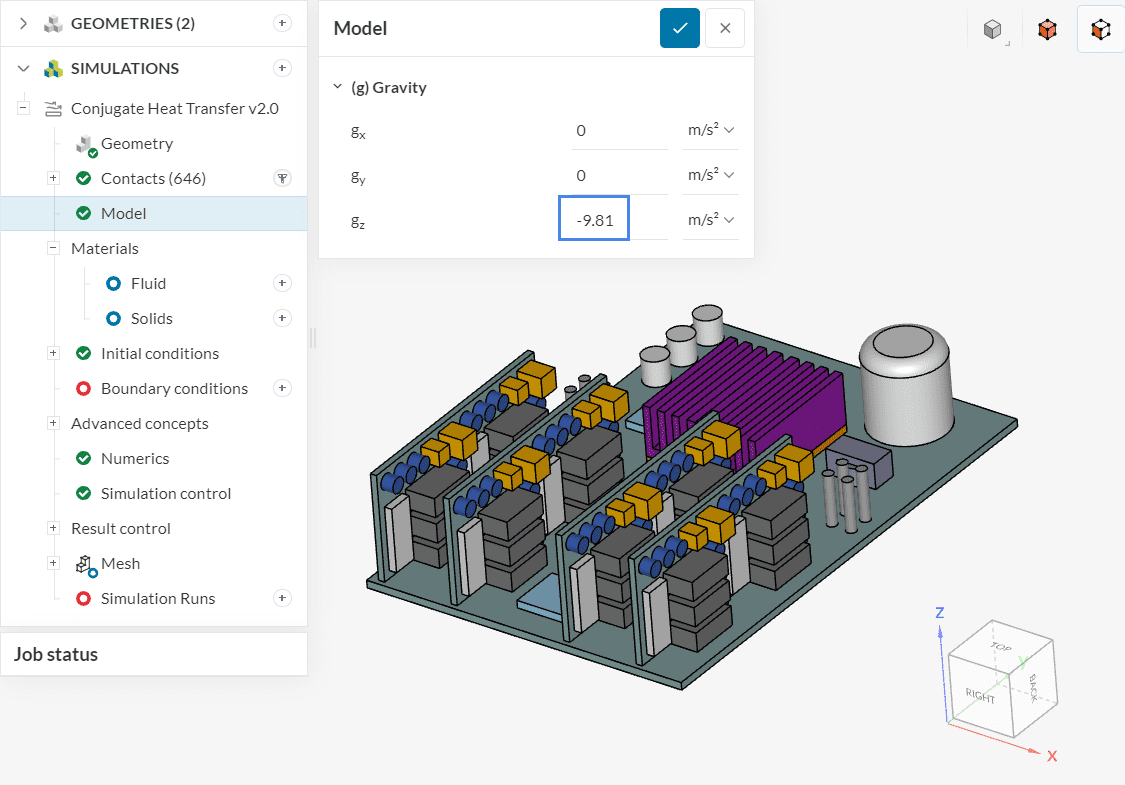
In this tutorial, gravity will be ‘-9.81’ \(m/s^2\) in the z-direction. The gravity definition is even more important when dealing with natural convection.
2.6 Materials
The next step in the setup is the material assignment for the various components of the electronic box. In the table below, you will find a summary of the material assignments.
| Material | Saved Selections |
| Air | Fluid Volume |
| Aluminum | Housing |
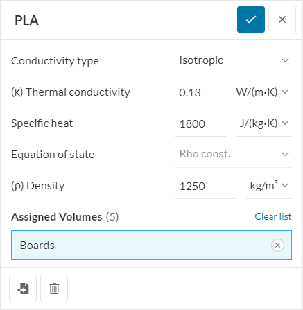
| PLA | Boards |
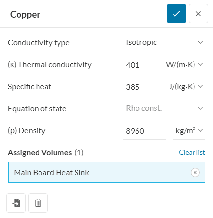
| Copper | Main Board Heat Sink |
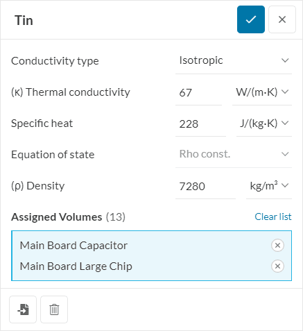
| Tin | Main Board Large Chip, Main Board Capacitors |
| Silicon | Board Flat Chip, Board Chips, Board Capacitors, Small Chips, Transformer, Board Large Chip, Board Large Chips |
In this tutorial, all materials will keep the default settings. However, it is possible to use custom materials in SimScale, as described in this article.
1. Fluid Materials (Air)
To define a new fluid, click on the ‘+’ next to the Fluids item. Doing so makes the fluid library pop up:
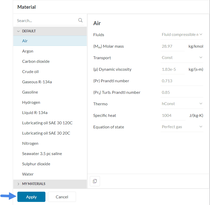
Choose ‘Air’ and hit ‘Apply’ to confirm the selection. Next, the material properties pop up:
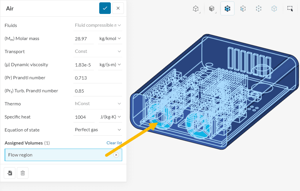
After assigning the flow region to the air domain, we will take care of the materials for the electronic components. For better visualization of the next steps, it’s recommended to hide the already assigned parts, therefore hide the Fluid Volume by clicking on the eye icon in the list of Saved Selections.
Be careful when assigning solid materials
When creating and assigning materials beware of what parts of the geometry are highlighted, because this will be assigned to the new material automatically.
Also, note that every part in the CAD model needs to be assigned to one and only one material.
2. Solid Materials (Aluminium)
Next, we select the solid material for the housing. For this tutorial, we will use the aluminum material provided by SimScale. The following list will be visible after clicking on the ‘+’ button next to Solids:
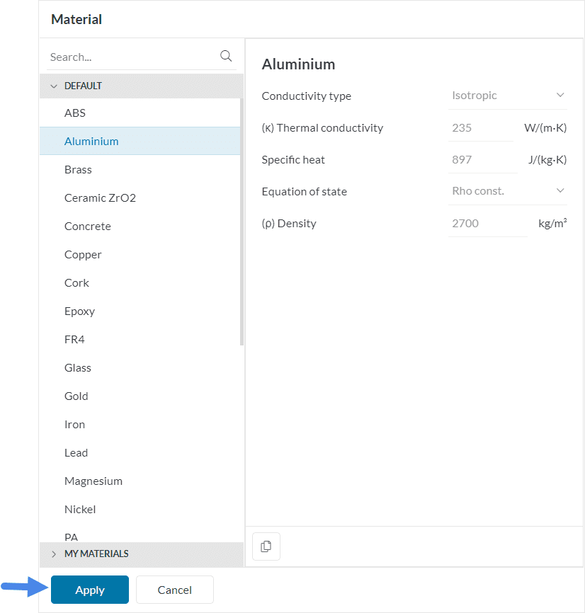
From the list, select ‘Aluminium’ and hit ‘Apply’ to confirm.
Next, we have to select the part which we want to assign to the Aluminium material. To do this either select the ‘Housing’ from the Saved Selections or select the part directly in the user interface.
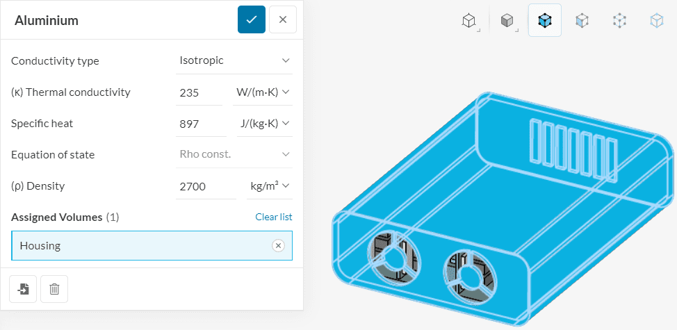
Remember that you can hide the Housing volume after the assignment to make the next steps easier.
3. Solid Materials (PLA / Copper / Tin / Silicon)
Next, following Table 1, we will assign the rest of the solid materials. Therefore repeat the steps for the Aluminum material assignment and select the equivalent material from the material library. The results for each material should look like this:
PLA (Polylactic Acid)
Copper
Tin
Silicon
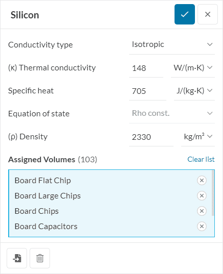
For the Silicon assigned volumes, not all Saved Selections are visible in the figure above. Please make sure to also assign the ‘Small Chips’ and ‘Transformer’ sets.
Custom Material
If you are looking for materials with different settings than the default values, you can always create custom materials:
2.7 Initial Conditions
Initial conditions are the starting points for any simulation. We are going to leverage a subdomain initialization to define the initial temperature for the Main Board Large Chip and the Main Board Heat Sink. The intention is to initialize the volumes that dissipate heat with a temperature close to the expected result, which can improve the convergence rate of a simulation.
Therefore, create a subdomain for the initialization of temperature and assign the temperature and the parts.
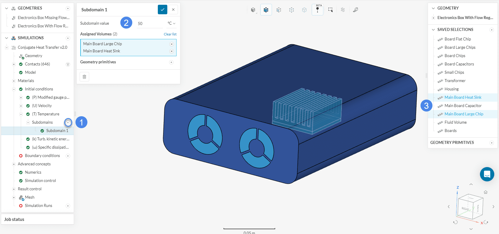
- Create a new temperature subdomain initialization by clicking the ‘+’ icon.
- Set the Subdomain value to ’50’ \(°C\).
- Assign the ‘Main Board Heat Sink’ and ‘Main Board Large Chip’ sets.
Did you know?
Changing the initialization of variables is not mandatory for a simulation, as SimScale’s default values work for most cases.
However, by using your knowledge about your application to provide better initial conditions, you can increase the convergence rate and improve the stability of the run.
2.8 Boundary Condition
Next, we have to assign the boundary conditions to the simulation. For this tutorial, we assume that the electronic box is equipped with external fans at the case outlets, which will suck the air through the electronics box.
2.8.1 Boundary Condition Overview
The following picture shows an overview of the physical situation applied in this electronics cooling tutorial:
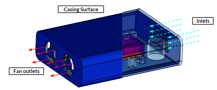
In this example, air movement is forced by fans sucking the air out of the domain. The casing surface helps to lose heat to the exterior domain via convection. In this example, we do not create an exterior domain to simulate the external heat transfer of the electronic box. We will assume the device to be in a 20 \(°C\) ambient environment and simulate the heat transfer to the ambient by applying an external wall boundary condition.
a. Fan Outlet
SimScale provides a fan boundary condition where the user can define a fan curve of interest. Please follow the steps below:
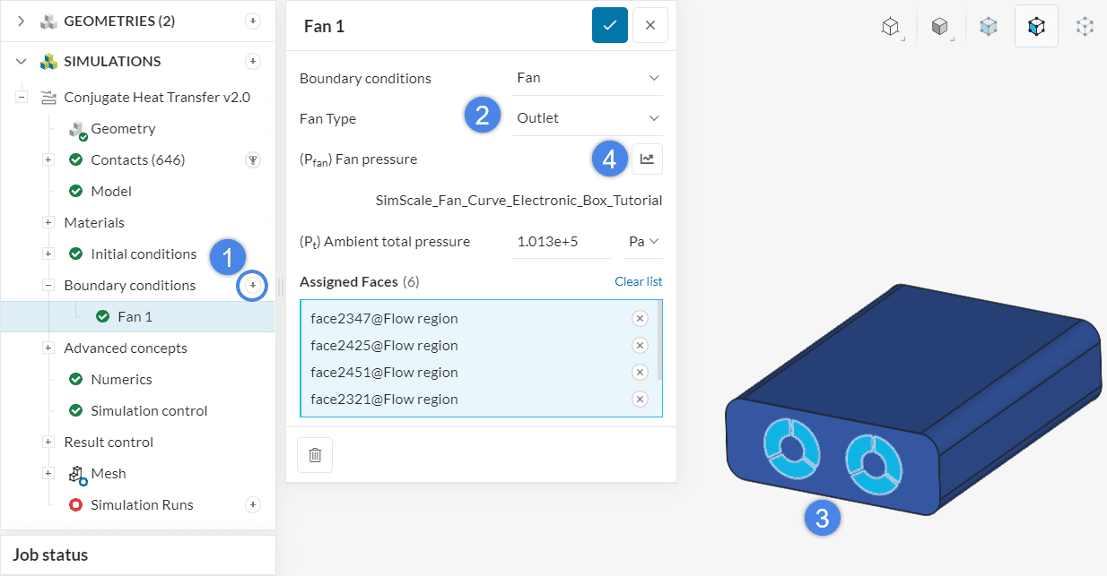
- Click on the ‘+’ button next to Boundary conditions and select ‘Fan’ from the list.
- Make sure that the Fan Type is set to ‘Outlet’ so the fan removes air from the flow region.
- Assign the 6 outlet faces to the boundary condition.
- Click on the graph icon to define the fan curve via table input.
In the table input window, you will be prompted to define volumetric flow rates and the corresponding fan pressures. Please download the CSV file using the link below, and upload it in the table configuration window:
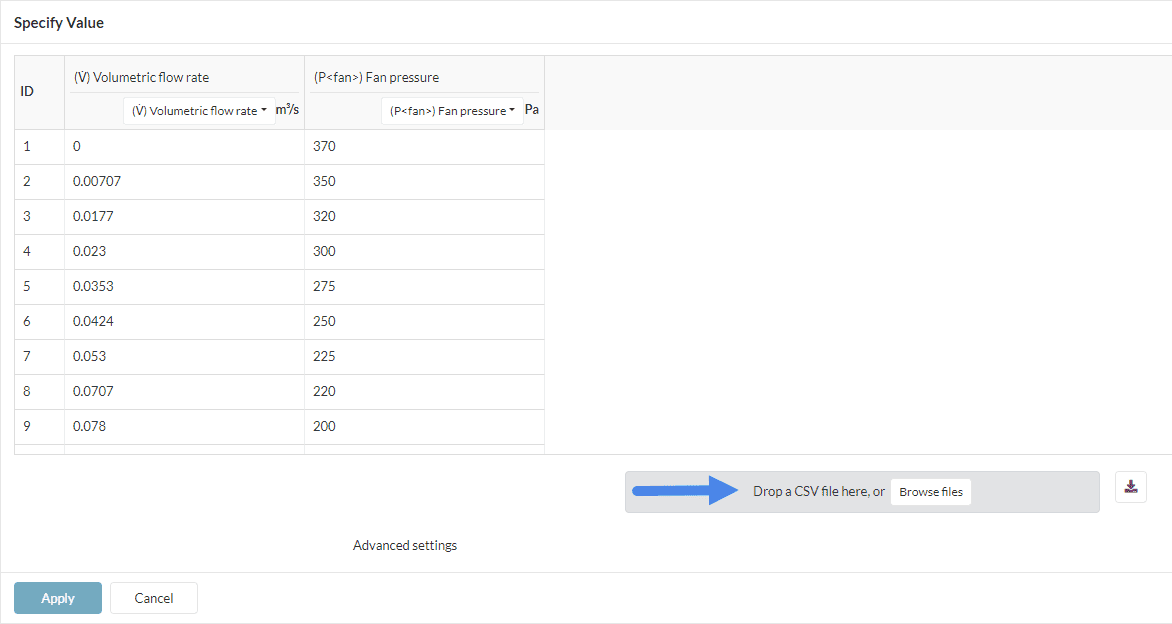
Once the CSV file is uploaded, press ‘Apply’ to save.
Did you know?
This tutorial covers the fan boundary condition workflow, however, it is also possible to use a velocity outlet if you are interested in a specific value for the flow rate at the outlet.
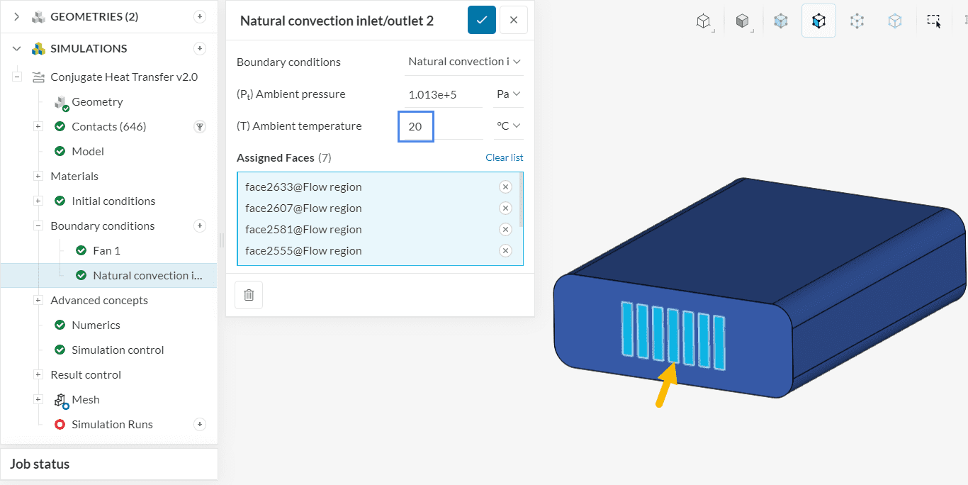
b. Inlet – Natural Convection Inlet Outlet
For the airflow into the electronic box, we will define a natural convection boundary condition. This boundary condition allows flow into or out of the domain, and it fixes the temperature value if the flow goes in.
Therefore, create a new boundary condition and select the ‘Natural convection inlet/outlet’ type. Adjust the Ambient temperature to ’20’ \(°C\) and assign it to the 7 inlet faces:
c. Thermal Wall – Housing
Lastly, we have to define the influence of the ambient temperature on the electronic box. Since we don’t simulate the airflow around the electronic box, we will use a thermal wall model for the external faces of the housing, responsible for accounting for the convective heat fluxes between the housing and the surrounding environment.
Create a new boundary, selecting ‘Wall’ as the type. The setup for the external wall heat flux model can be seen in the figure below:
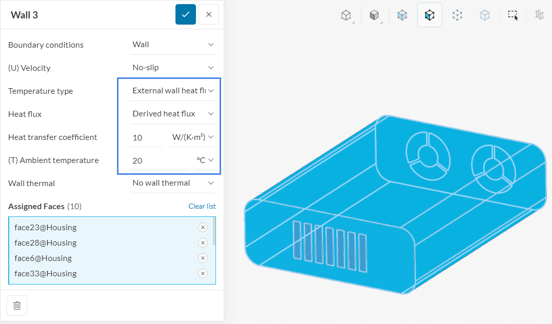
After creating a wall boundary condition, change the Temperature type to ‘External wall heat flux’. The Heat flux method will be ‘Derived heat flux’, which allows us to define a Heat transfer coefficient of ’10’ \(\frac {W}{k.m^2}\) and an Ambient temperature of ’20’ Celsius. All 10 external faces of the housing will receive this boundary condition.
Unassigned Surfaces
Surfaces that are not assigned to a boundary condition or a contact will be treated as an adiabatic wall. Therefore, such faces will be taken as a perfect thermal insulator, with no heat flux across the face.
2.9 Advanced Concepts – Defining Power Sources
Components in electronic devices receive electrical current and generate heat. Heat dissipation from any component can be defined as power sources. In this tutorial, we will only assign a power source to the main CPU and the other small chips.
The following table describes the power source and the Saved Selections.
| Saved Selections | Power Source \([W]\) |
| Main Board Large Chip | 60 |
| Small Chip | 0.8 |
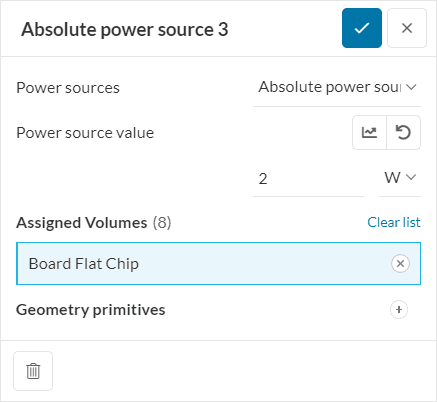
| Board Flat Chip | 2 |
The configurations of the individual power sources are described in the images below:
a. Main Board Large Chip
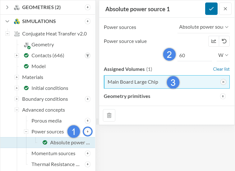
- Under Advanced concepts, hit the ‘+’ button next to Power sources and select ‘Absolute power source’.
- Define the amount of heat dissipation, which is ’60’ \(W\) for the main board chip.
- Assign the power source to the ‘Main Board Large Chip’.
Did you know?
You can assign as many different heat sources as you like. You also have the option to assign the power sources to a geometry primitive you define during the simulation setup, in case you do not have the electronic component generating heat represented in your model.
The following figures show the heat sources applied in this tutorial, please follow the same workflow as just described:
b. Small Board Chips
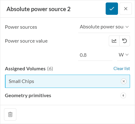
Keep in mind that, when defining an absolute power source for multiple volumes, the Power source value will be dissipated by each one of the assigned volumes.
c. Board Flat Chips
These advanced concepts might also be helpful for an electronics cooling application:
- Rotating zones: If your CAD model contains the rotor blades, you can set up their rotational properties here.
- Thermal resistance networks: Here you can define simplified thermal resistance networks that dissipate heat.
- Momentum sources: This serves as a simplification for modeling the fans, in case you do not have the fan’s geometry.
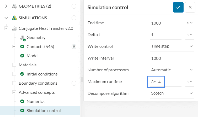
2.10 Simulation Control
The default settings for Numerics are usually suitable. Experienced users can use manual settings for smoother or faster convergence.
The Simulation Control settings define the general controls over the simulation. We will adjust the Maximum runtime to ‘30000’ seconds, to ensure that the simulation runs until the end of the 1000 iterations.
2.11 Result Control
As a default setting, velocity, pressure, density, temperature, and radiation variables will be saved for every cell in the fluid domain. The changes of those between the timesteps are displayed in the convergence plot.
You can use result control to observe the development of the values at any point or surface in your domain during the calculation. For this tutorial, we will create two result control items to analyze the airflow through the electronic box.
2.11.1 Outlet Temperature
To evaluate the temperature of the air at the outlet, create an area average on the outlet faces. With that, the physical data for these surfaces such as pressure, temperature, velocity, and more will be tracked for every iteration. Follow the steps presented in the figure below:
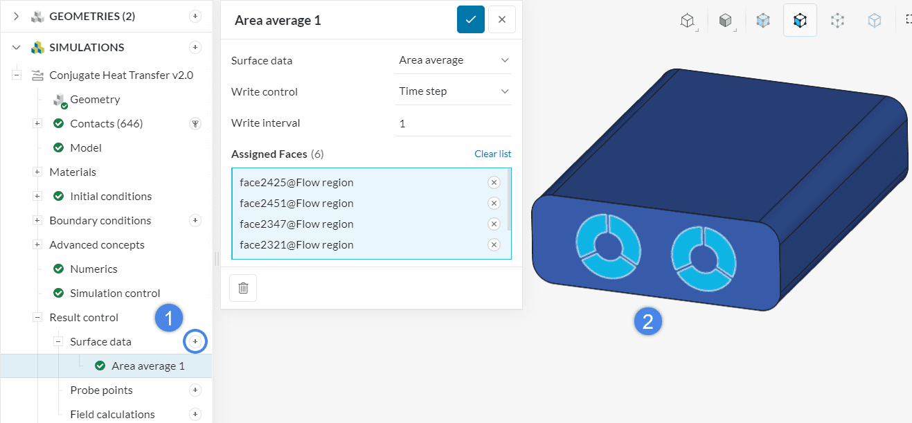
- Hit the ‘+’ button next to Surface data under Result control and choose an ‘Area average’.
- Assign it to the six outlet faces.
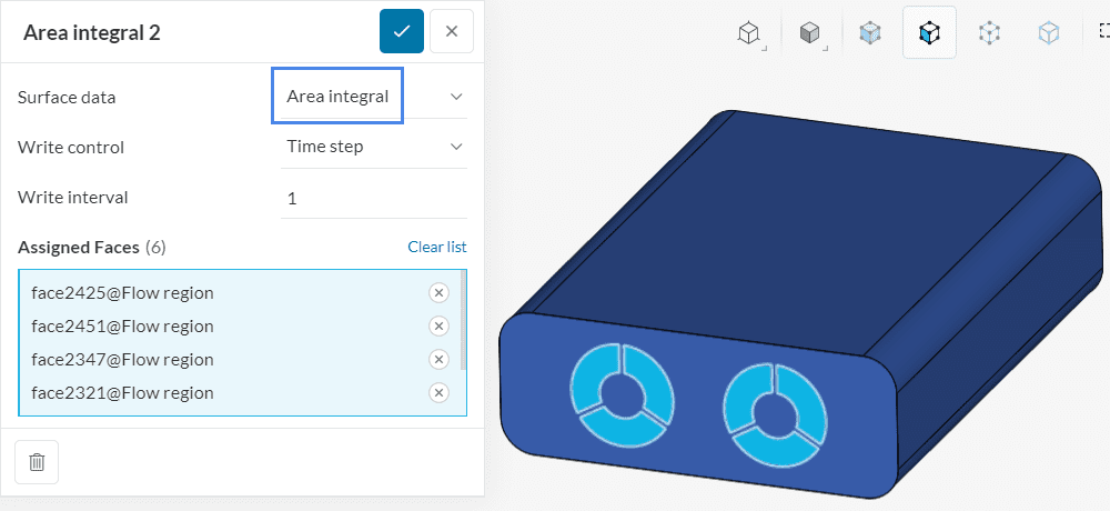
2.11.2 Volumetric Flow Rate
Following a similar workflow, create a new surface data result control, but this time choose ‘Area integral’. This result control integrates the fields on faces of interest, therefore it helps evaluate volumetric flow rates.
Assign the 6 outlet faces to the result control, as below:
As a rule of thumb, it is a good idea to use result controls to keep track of parameters of interest in the simulation domain. For example, flow rates, pressure drops, the temperature of certain surfaces, etc. are some commonly used options.
2.11.3 CPU Temperature
The last result control is an ‘Area average’ assigned to the top face of the Main board large chip. With this result control, we will keep track of the average temperatures experienced on the chip.
3. Mesh
Default mesh settings usually create a good initial mesh. For this tutorial, most of the default mesh settings will be kept, as shown below:
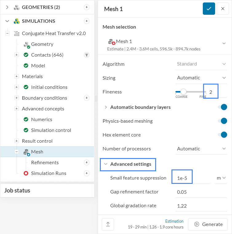
From the global settings, adjust the Fineness to ‘2’ and the Small feature suppression (under Advanced settings) to ‘1e-5’ meters.
Did you know?
The standard meshing tool offers many options for customization, including several mesh refinements and further fine-tuning. Interested users are encouraged to visit this page.
4. Start the Simulation
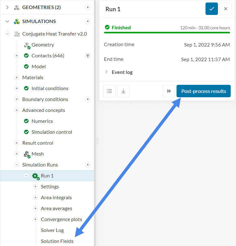
After all the settings are completed, click on the ‘+’ icon next to Simulation Runs, to start with the analysis. This way, the mesh will be generated and the simulation run will start automatically afterward.
While the results are being calculated, you can already have a look at the intermediate results in the post-processor. They are being updated in real-time!
5. Post-Processing
When the simulation is complete, you can check the Convergence plot and the Solution fields from the simulation. You can access either of them in the simulation tree by clicking on them, as you can see below:
5.1 Convergence and Outlet Flow Temperature
When the simulation is running and after its completion, we can observe the convergence behavior. For a steady-state analysis, the result should converge to a point where the flow field characteristics do not change anymore.
a. Convergence Plot
For each timestep, the solver calculates solutions for each cell in the mesh. The residuals are the differences between those results. Hence the lower the residuals, the more stable the solutions are. We also call that “convergence”. The following picture shows the convergence plot for the solution variables.
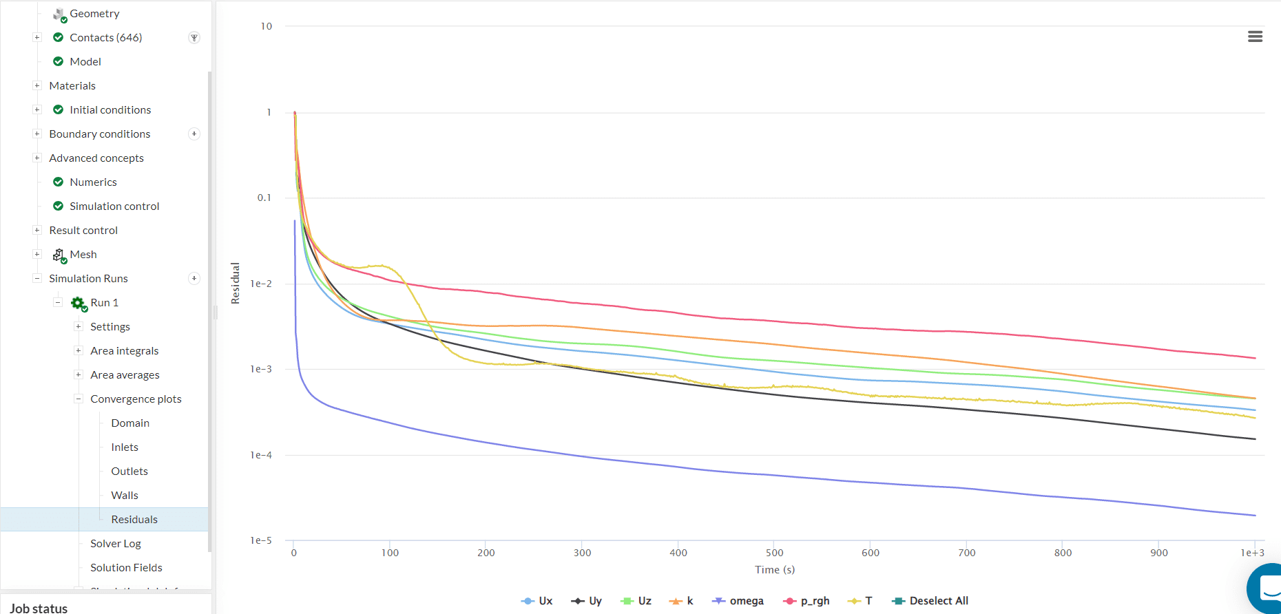
- Select the finished Simulation run.
- Open convergence plots and residuals.
The residuals are presented dimensionless and you can convert them into a percentage: In the tutorial, all graphs are beneath 1e-2 and some even lower than 1e-3, which is a good sign for convergence.
b. Result Control
With the result control items created we can analyze the results for special faces of interest. The outlet temperature is a good physical parameter to track to evaluate convergence and the performance of the design. The result for the temperature of each outlet face can be seen below.
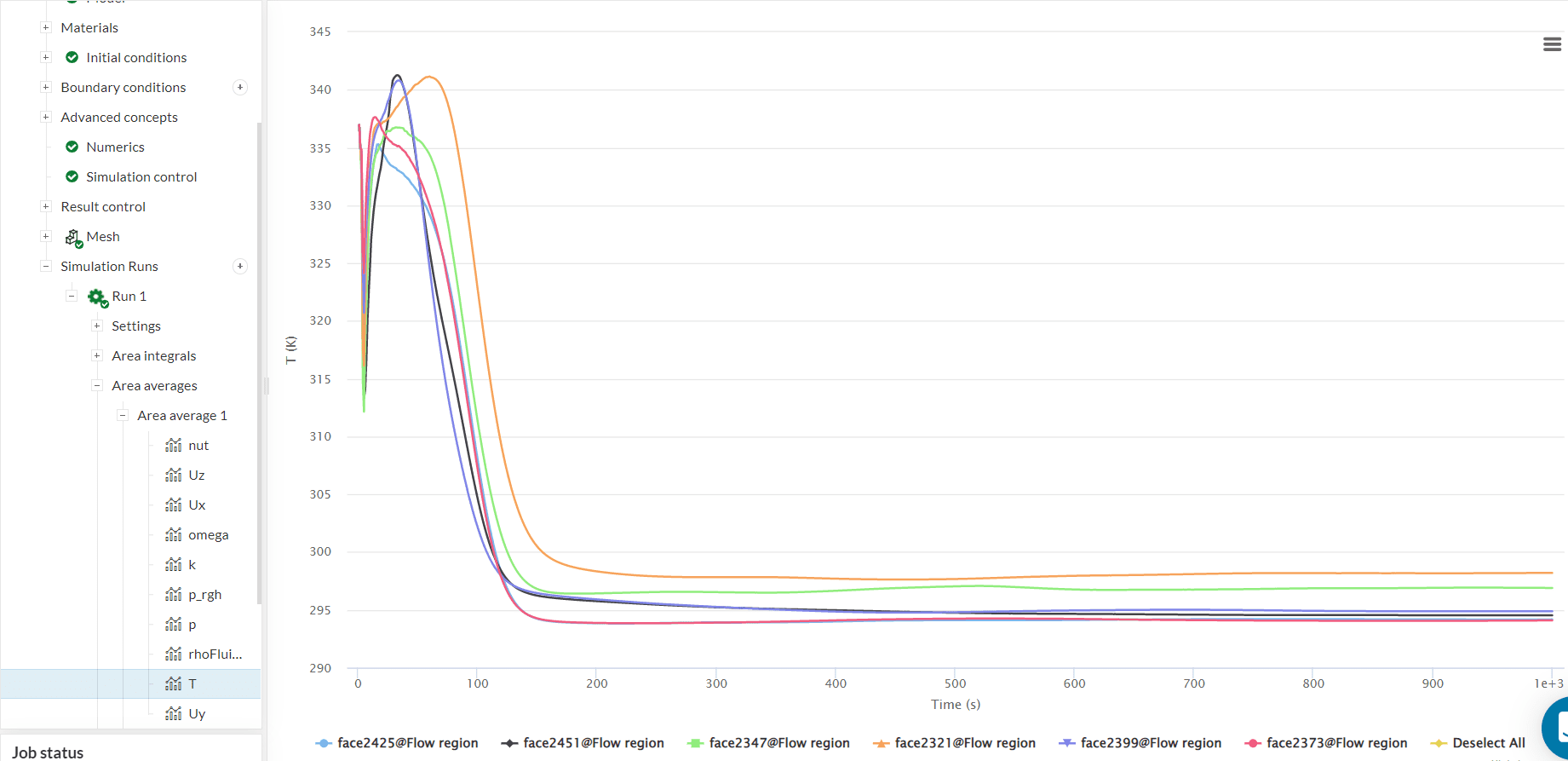
Having a look at this plot, most of the temperatures approach a horizontal line, which means, that the result is approaching a steady-state result. The maximum temperature is 298.2 \(K\) ( 25 \(°C\)). Averaging the temperature for all faces we get an average outlet temperature of 295.4 \(K\) (22.2 \(°C\)), which means we have an increase of 21 \(K\) between the inlet and the outlet.
5.2 Surface Visualization
Let’s have a look at the different temperatures and the flow field visually. This can either be done by selecting ‘Solution Fields’ in the simulation tree or ‘Post-process results’ from the run panel.
5.2.1 Main Board Temperature
At first, we will have a look at the temperature of the Main Board. Therefore hide the cutting plane and choose ‘Temperature’ to display on the Parts Color Coloring. Change the units to \(°C\). To improve the quality of your visualization by making the color transition smoother, right-click on the legend bar at the bottom, and select the ‘Use continuous scale‘ option as shown in step 3 below:
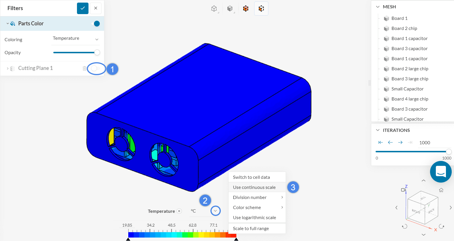
- Toggle off the visibility of the cutting plane.
- Switch the temperature units to ‘\(°C\)’.
- Right-click on the temperature scale and select a continuous scale.
You can hide the outer parts and have a look at the chips inside. For example, to visualize the internal parts, hide the ‘Housing‘ on the geometry tree list. Alternatively, you can activate the parts selection, select the housing, and right-click to hide the selection.

We can see how the temperature not only affects the parts but also the mainboard PCB.
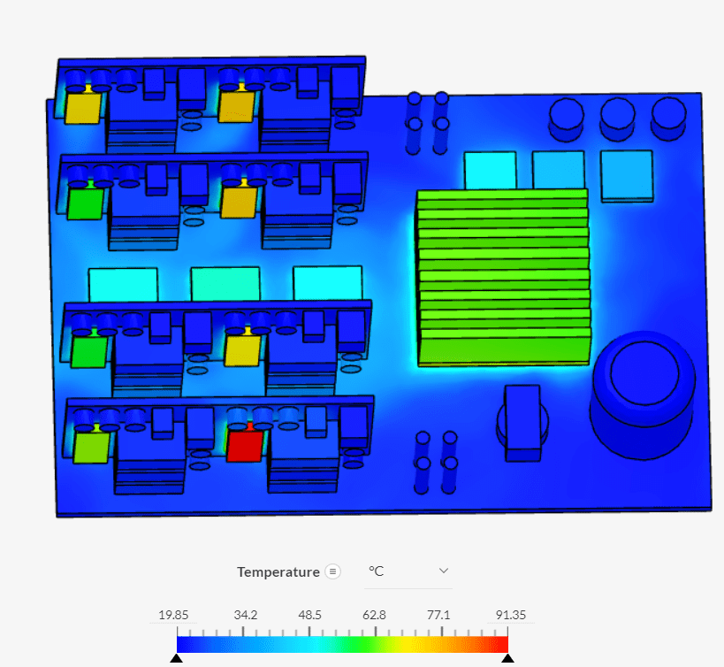
We can see that the temperature of the chips closer to the outlets is quite high. This makes sense because they are not exposed to the middle of the flow. Furthermore, some heat has already been transferred to the air at the beginning of the flow domain, so its capacity to lower the temperature has decreased.
5.3 Cutting Plane
Next, we want to take a look at a section of the electronics box.
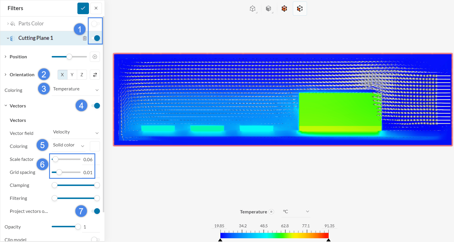
- Toggle off the Parts color to hide all the parts and toggle on the Cutting Plane to make it visible.
- For the Orientation, choose the ‘X‘ axis. It will automatically generate a plane normal to this axis, coincident with the origin of the model.
- Choose ‘Temperature’ as the Coloring parameter.
- Toggle on Vectors.
- Switch the Coloring to ‘Solid color’ and choose white color.
- Set the Scaling factor to ‘0.06’ and the Grid Spacing to ‘0.01’.
- Enable the Project vectors onto plane option.
With this kind of visualization, we can get insights into the flow field internal to the box.
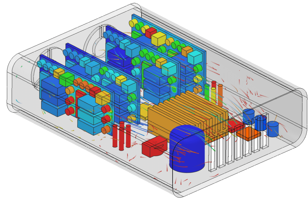
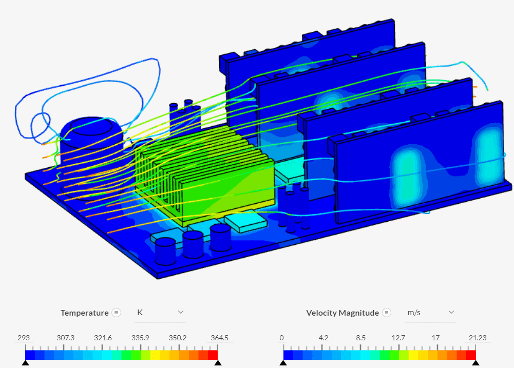
5.4 Streamlines
Finally, to view the streamlines, add a ‘Particle Trace’ filter. Keep in mind that you need to activate the visibility of the parts coloring to use the openings as seed faces. You can also toggle off the cutting plane, as it won’t be needed for the particle traces filter.
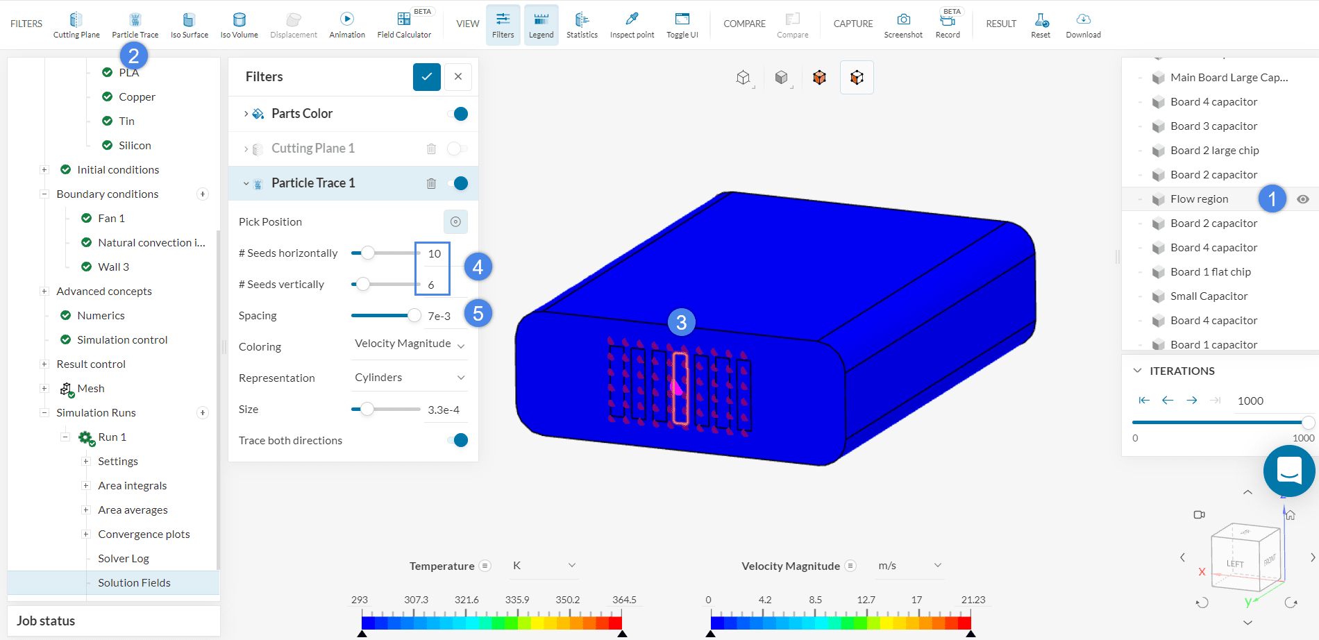
- Ensure that the Flow region volume is visible
- Create a new ‘Particle trace’ by selecting the icon from the filter section
- Select one of the inlet faces as a seed for the traces
- Adjust the # Seeds horizontally and # Seeds vertically to roughly cover the inlet faces
- Set the Spacing to ‘0.007’ so that the seeds are spaced out
After finishing the setup, and hiding the housing and flow region, the result should look similar as presented in the figure below.
For a general overview of SimScale’s online post-processing capabilities, this documentation can be used.
Congratulations! You finished the tutorial!
Note
If you have questions or suggestions, please reach out either via the forum or contact us directly.
Last updated: April 6th, 2026
Did this article solve your issue?
How can we do better?
We appreciate and value your feedback.


