What is Thermal Expansion?
Thermal expansion is the increase of the geometric dimensions (length, area, volume) of matter as its temperature is increased. The reversal of this process due to cooling is often referred to as thermal contraction. The characteristic value describing this behavior is the thermal coefficient of expansion which is expressed as the fractional change in length or volume divided by the change in temperature.
Heating a material makes its particles move faster and the intermolecular forces between them weakens. This leads to an increase in the average separation between atoms and molecules which manifests on a macroscopic level as an expansion of the geometric dimensions and a reduction of the material’s density. Some materials, however, experience contraction with increasing temperature within limited temperature ranges. Although this behaviour is the exception, there are some commonly known examples, like water between 0 °C and 4 °C.
Applications and Examples of Thermal Expansion
A common everyday example of thermal expansion is mercury, alcohol, or liquid-in-glass thermometers. When the temperature increases, the liquid expands and moves up the thermometer’s capillary. Another common example is a hot-air ballon, where the expanding hot air’s lower density exerts an upward force making the hot air ballon float.
However, thermal expansion often poses a risk in many engineering applications. In closed hydraulic and water heating systems, for example, thermal expansion tanks are necessary components which absorb the volume changes of the hydraulic fluid between minimum and maximum temperature and thus keep the pressure largely constant.
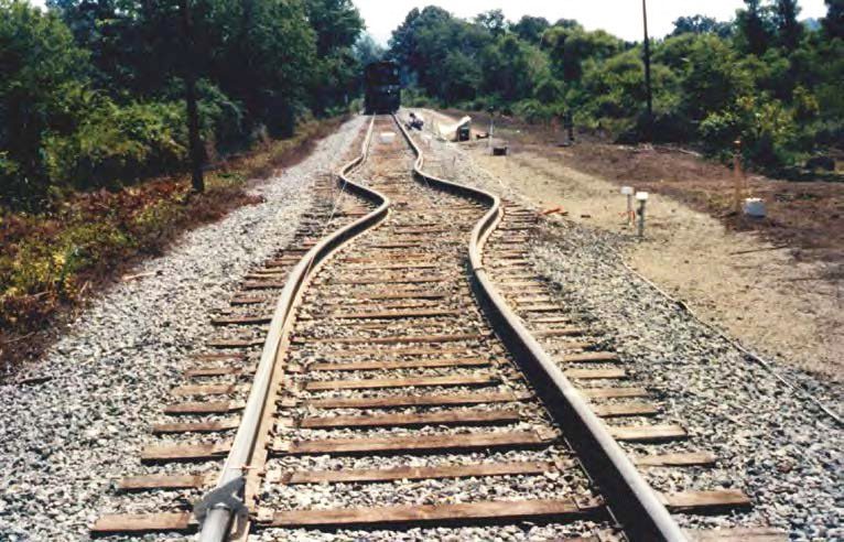
Similarly, thermal expansion in solids can be a significant hazard, especially in the AEC industry. Railway tracks can buckle due to the compressive stresses caused by thermal expansion when heated by the sun. These so-called “sun-kinks” are shown in Fig. 1 and can cause a train to derail. In this video, shot from inside a railway engine, we can see how scary it is when a train drives over kinks in the track.
Similar susceptibilities exist in buildings, pipelines, roads and bridges during hot weather. Expansion joints, as the one shown in a bridge in Figure 2, accommodate thermal expansion to prevent damage or buckling.

Therefore, thermal expansion must be well-understood in engineering efforts involving heat transfer and high temperatures.
Mathematical Description of Thermal Expansion
Changes in temperature lead to changes in the volumes of solids and liquids. To quantify this phenomenon, we use a material and temperature-dependent thermal expansion coefficient γ defined as
$$\gamma = \frac{1}{V_0} \left (\frac{\partial V}{\partial T} \right )_\mathrm{p}\tag{1}$$
For small changes in temperature, the change in relative volume \(\frac{\Delta V}{V_0} = \frac{V-V_0}{V_0}\) and the change in temperature \(\Delta T = T – T_0\) are approximately linearly related, such that we can define a mean thermal expansion coefficient:
$$ \bar \gamma = \frac{\Delta V}{(V_0)(\Delta T)}\tag{2}$$
Three different types of coefficients have been developed, namely volumetric, areal, and linear. In solids, we can simplify the problem to linear expansion where we consider a change in one dimension as opposed to a change in volume. In this case, the change in length is related to the temperature change by a coefficient of linear thermal expansion:
$$ \alpha = \frac{1}{L_0} \left (\frac{\partial L}{\partial T} \right )_\mathrm{p} , \bar \alpha = \frac{\Delta L}{L_0 \Delta T}\tag{3}$$
The estimation of the mean coefficient of linear thermal expansion works well as long as the coefficient does not change much with the temperature and the change in length is small \(\frac{\Delta L}{L} \text{«} 1\). Solids, for the most part, show little dependence of the coefficient on temperature. Three For isotropic materials, the volumetric thermal expansion is three times the linear coefficient \(\bar \gamma = 3 \bar \alpha\). The coefficient is almost always positive. In the rare cases where a material contracts with increasing temperature, the coefficient becomes negative.
Values of linear coefficient of thermal expansion for different materials
Tab. 1 lists the linear coefficient of thermal expansion for common engineering materials.
| Material | Linear Coefficient of Thermal Expansion [ \( \times \) 10-6/°C] |
| ABS | 80 |
| Aluminum | 23 |
| Brass | 17-21 |
| Ceramic ZrO2 | 10.5 |
| Concrete | 10 |
| Copper | 16.5 |
| Cork | 40 |
| Epoxy | 50 |
| FR4 | 14 |
| Glass | 9 |
| Borosilicate glass | 3.3 |
| Gold | 14 |
| Granite | 4.4 |
| Ice | 28 |
| Invar | 0.6-2.1 |
| Iron | 11.8 |
| Ductile high-chromium cast iron | 9.3–9.9 |
| Iron-cobalt-nickel alloys | 0.6–8.7 |
| Magnetically soft iron alloys | 2.0–12 |
| Lead | 28 |
| Magnesium | 25 |
| Nickel | 13.4 |
| Platinum | 8.8–9.1 |
| PA6 (Nylon 6) | 91 |
| PA6 GF30 | 20-30 |
| PA66 GF30 (Nylon 66) | 20-30 |
| Polyethylene (HDPE) | 169 |
| Polypropylene (PP) | 194 |
| Polyoxymethylene (POM) | 95 |
| Poly(methyl methacrylate) (PMMA) | 69 |
| Polystyrene (PS) | 71 |
| Polytetrafluoroethylene (PTFE) | 119 |
| Polyvinyl chloride (PVC) (at 50 °C) | 75 |
| Rubber | 6.7 |
| Silicon | 2.6–3.3 |
| Silver | 19 |
| Stainless Steel | 9.3-25 |
| Steel | 8.6-19 |
| Structural steel | 12 |
| Titanium | 8.5 |
| Unalloyed or low-alloy titanium | 7.6–9.9 |
| Tungsten | 4.5 |
Thermal stress analysis
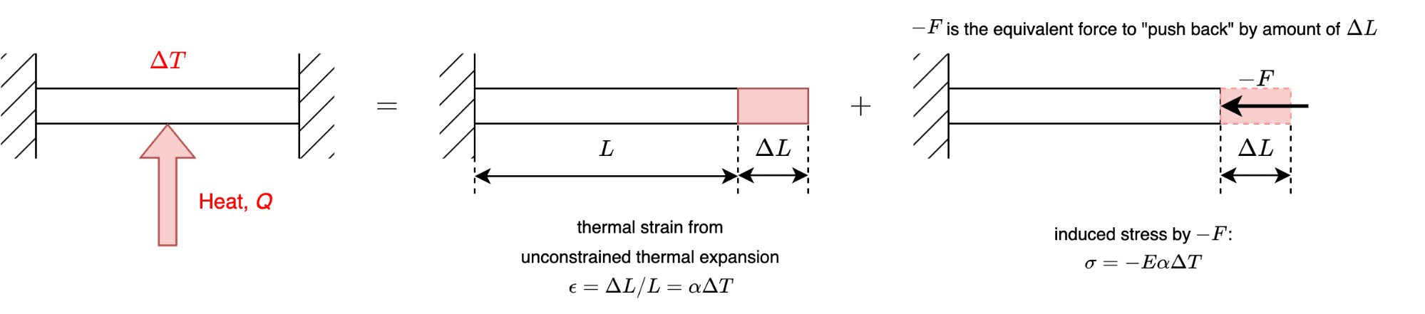
Thermal stresses in structures arise when the temperature rises uniformly in solids with physical constraints. A uniform-temperature increase in a beam with fixed ends will induce compressive stresses equal to \(\sigma = E \epsilon_T – \alpha E \Delta T\). We derive this by the following superposition of the situations:
Non-uniform temperature distribution can also induce thermal stresses which in turn leads to non-uniform thermal expansion within the material. The general thermomechanical case involves a solid with partial mechanical constraints coupled with non-uniform temperature distributions. The temperature distribution, in this case, is described with:
$$ \frac{\partial}{\partial x} \left (k \frac{\partial T(x,y,z,t)}{\partial x} \right ) + \frac{\partial}{\partial y} \left (k \frac{\partial T(x,y,z,t)}{\partial y} \right ) + \frac{\partial}{\partial z} \left (k \frac{\partial T(x,y,z,t)}{\partial z} \right ) + Q(x,y,z,t) = \rho c \frac{\partial T(x,y,z,t)}{\partial t}\tag{4}$$
The solution of the above equation is a necessary step preceding the thermal stress analysis of the solid figure shown in Figure 4. The first step in a thermal stress finite element analysis is the solution of the heat flow equation to calculate the temperature field. Subsequently, the temperature field is used as an equivalent to a body force to carry out the stress analysis.
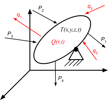
Figure 4 shows a solid with a temperature field distribution T(x, y, z, t) produced by thermal fluxes \(q_1, q_2, q_3, … \) and a heat source or sink represented by Q. The solid is also subject to mechanical forces \(P_1, P_2, P_3, P_4, … \). If we discretize the solid into finite elements, we can describe the strain of the elements as:
$$\begin{Bmatrix}\epsilon\end{Bmatrix} = \begin{Bmatrix}\epsilon _\mathrm{M}\end{Bmatrix} + \begin{Bmatrix}\epsilon _\mathrm{T}\end{Bmatrix}\tag{5}$$
\(\begin{Bmatrix}\epsilon _\mathrm{M}\end{Bmatrix}\) is the strain induced due to mechanical forces and stresses:
$$\begin{Bmatrix}\epsilon _\mathrm{M}\end{Bmatrix} = \begin{bmatrix}D\end{bmatrix}^{-1}\begin{Bmatrix}\sigma\end{Bmatrix}\tag{6}$$
\(\begin{bmatrix}D\end{bmatrix}^{-1}\) is the inverse of the materials stiffness matrix. \(\begin{Bmatrix}\epsilon _\mathrm{T}\end{Bmatrix}\) is the strain induced by the temperature change due to heat fluxes and heat sources:
\(\begin{Bmatrix}\epsilon _\mathrm{T}\end{Bmatrix} =
\begin{pmatrix}
\epsilon _\mathrm{T,xx} \\
\epsilon _\mathrm{T,yy} \\
\epsilon _\mathrm{T,zz} \\
\end{pmatrix} =
\begin{pmatrix}
\alpha \Delta T \\
\alpha \Delta T \\
\alpha \Delta T \\
\end{pmatrix}\tag{7} \)
After a bit of math, detailed in Sources [1-3], we arrive at the well-known element equation:
$$\begin{bmatrix}K_\mathrm{e}\end{bmatrix} \begin{Bmatrix}\Phi\end{Bmatrix} = \begin{Bmatrix}f_\mathrm{M}\end{Bmatrix} + \begin{Bmatrix}f_\mathrm{T}\end{Bmatrix} \tag{8}$$
In this manner, thermal expansion is incorporated into the finite element method.
Thermomechanical Analysis in SimScale
The Thermomechanical module in SimScale couples the effects of structural loads and thermal expansion. It enables you to virtually test and predict the behavior of structures and hence solve complex structural engineering problems subjected to static and thermal loading conditions. The FEA simulation platform uses scalable numerical methods that can calculate mathematical expressions that would otherwise be very challenging due to complex loading, geometries, or material properties.
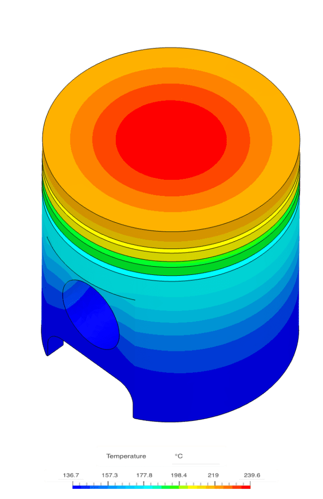
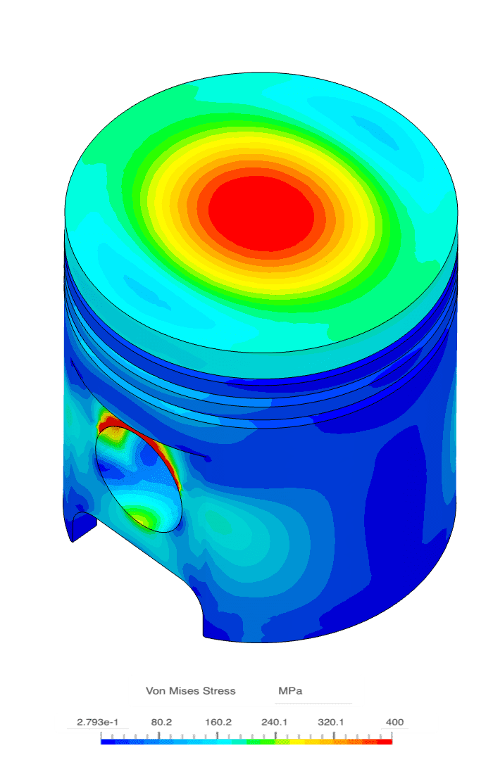
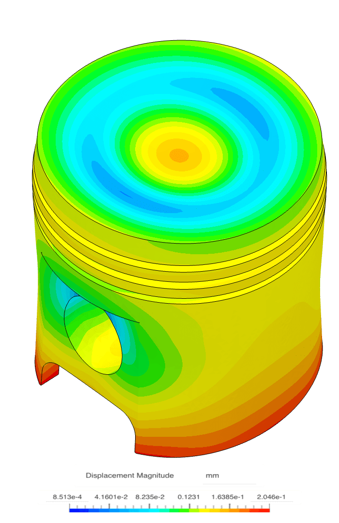
You can try the Thermomechanical module on SimScale by creating an account and following this tutorial on a simulation of an engine piston. In the figure below, you see the results from the tutorial. On the left, is the temperature field, while in the middle we see the stress distribution. We can see how the stresses correlate with the temperature gradients, especially on the top of the piston head. On the right, is the deformation (20x scale). These simulations are very easy to set up and any user can run several such simulations in parallel to quickly generate useful results.
With our cloud-native simulation platform, we empower every engineer to innovate faster by making high-fidelity engineering simulation technically and economically truly accessible at any scale.
Happy simulating!
References:
[1] Logan, Daryl, A First Course in the Finite Element Method, Chapter 15: Thermal Stress, Cengage Learning, 2012.
[2] Hsu, Tai-Ran, The Finite Element Method in Thermomechanics, Chapter 3: Thermoelastic-plastic Stress Analysis, Allen and Unwin, 1986.
[3] Hsu, Tai-Ran, Lecture Notes on Thermal Stress Analysis of Solid Structures Using Finite Element Method, Introduction to Finite Element Method, San Jose University, 2017.
[4] ASM Ready Reference: Thermal Properties of Metals, Chapter 2: Thermal Expansion, ASM International, 2002.
[5] VDI Heat Atlas, Chapter D6: Properties of Solids and Solid Materials, Springer, 2010.
Last updated: February 20th, 2023
Did this article solve your issue?
How can we do better?
We appreciate and value your feedback.
What's Next
What is Conduction?

