What is Heat Flux?
Heat flux, sometimes referred to as thermal flux, is a flow of energy per unit area and per unit time. It is typically measured through a solid surface, as in the case of conduction heat transfer. It can also be measured at a fluid-solid boundary; this is typical of a convective heat transfer analysis, where the Nusselt number relates the wall heat flux to the temperature difference. In other words, it quantifies the amount of heat transferred through a surface in a specific direction. Engineers and product designers often encounter heat flux considerations in the design and optimization of systems where heat transfer is a critical factor, such as electronic devices, HVAC systems, and industrial processes.
The SI units of heat flux are Watts per square meter \((W/m^2)\). Heat flux is a vector quantity, as it has both a magnitude and direction.
Heat Flux Theory
Fourier’s Law
At the heart of the concept of heat flux lies Fourier’s law of heat conduction, named after the French mathematician and physicist Jean-Baptiste Joseph Fourier. It essentially defines the equation of heat flux. Fourier’s Law states that the rate of heat transfer through a material is proportional to the negative gradient in the temperature and area. It underscores the fundamental relationship between heat flux and the factors influencing it. The negative sign indicates that heat flows in the direction of decreasing temperature, following the natural tendency for heat to move from higher to lower temperatures.
Fourier’s law can be stated in both differential and integral forms. The integral form states the amount of energy flowing into or out of the surface of a body and, therefore, is very applicable to experimental systems.
Differential Form of Fourier’s Law
Fourier’s law in one dimension:
$$ q_x = – k \frac{dT}{dx} $$
Where:
\(q\) = local heat flux density, \([W/m^2]\)
\(k\) = material thermal conductivity, \([W/(m.K)]\)
\(T\) = temperature \([K]\)
\(x\) = distance in x direction \([m]\)
Understanding the temperature gradient is pivotal in grasping the nuances of heat flux. The temperature gradient (\(\frac{dT}{dx})\) represents how the temperature changes concerning the distance traveled. A steep gradient implies a rapid change in temperature over a short distance, intensifying the heat flux. Conversely, a shallow gradient corresponds to a gradual change in temperature, resulting in a lower heat flux.
Similarly, the thermal conductivity (\(k)\) of a material plays a pivotal role in determining how well it conducts heat. Materials with high thermal conductivity facilitate efficient heat transfer, making them suitable for applications where minimizing thermal resistance is crucial. In contrast, materials with low thermal conductivity may be chosen to insulate against heat transfer.
Engineers must consider these material properties when selecting components for their designs, aligning with the principles embedded in Fourier’s law and the heat flux equation.
Integral Form of Fourier’s Law
$$ \frac{\partial Q}{\partial t} = – k \oint\oint \nabla T \cdot dS $$
Where:
\(\frac{\partial Q}{\partial t}\) = amount of heat transferred per unit time \(W\)
\(dS\) = surface area vector \([m^2]\)
How to Measure Heat Flux
Accurate measurement of heat flux is crucial for designing effective thermal management systems. To measure heat flux, you can follow different physical measurement methods, including:
- Heat Flux Sensors: These devices directly measure the heat transfer across a surface. Thin, thermally conductive materials with embedded thermocouples or resistance temperature detectors (RTDs) provide real-time data.
- Calorimetry: This method involves measuring the temperature change in a substance due to heat transfer. By monitoring the mass, specific heat, and temperature change, engineers can calculate heat flux.
- Infrared Thermography: Infrared cameras detect surface temperatures and, combined with material properties, enable the calculation of heat flux.
However, heat flux can be estimated and analyzed much earlier in the design cycle of a product or part. For this, engineers can leverage the power of engineering simulation, particularly cloud-native simulation.
Heat Flux Simulation and Analysis
With simulation, you can visualize the heat flux and identify areas of concern that can inform your design decisions and enable you to optimize your design quickly. With SimScale’s cloud-native thermal simulation tools, you can run multiple thermal simulations in parallel by taking advantage of the cloud’s infinite computing and storage capabilities. This allows for design parametrization and accelerated design innovation. You may also run multiple physics simulations, combining thermal simulations with structural, flow, and electromagnetics simulations that provide you with a comprehensive analysis of your design all in one place – your web browser. In the following chapter, we take a deeper look at how heat flux is simulated and visualized in SimScale.
Heat Flux Measurement in SimScale
Heat Flux is available as a boundary condition, global result field, and surface result control within SimScale. It is available in both Conjugate Heat Transfer/IBM (CFD) and Heat Transfer (FEA) analysis types.
Heat Flux Boundary Condition
Heat flux can be defined as an input parameter to a simulation, also known as a boundary condition. Within the Conjugate Heat Transfer (CHT) analysis type, it can be defined via a Wall boundary condition. Note that a thermal flux wall boundary condition should only be applied on an external surface of the domain, and it is incorrect to define it on an internal surface. If a heat load on a body inside the domain needs to be defined, this should be done via a Power source.
The default temperature definition on a wall boundary condition is Fixed value; however, this can be changed to External wall heat flux. From there, there are 3 options for heat flux definition. A Fixed heat flux definition has units of power per unit area (W/m2). Fixed power allows the user to define a value in absolute Watts; it is not a function of the area. A Derived heat flux allows the user to define a Heat transfer coefficient or film coefficient. A Derived heat flux allows the user to define a heat transfer coefficient and reference temperature. The heat transfer units are Power/Temperature delta*Area \((W/(K.m^2\)).
The actual heat flux is dependent on the temperature of the wall. For example, if a 1 \(m^2\) wall with a convection coefficient of 5 and a reference temperature of 20 \(°C\) has an average temperature of 30 \(°C\), there will be 50 Watts of heat transfer through that surface.
For both Fixed power and Fixed heat flux, a positive value indicates heat is being added to the selected surface; a negative value means heat is leaving the system. A Derived heat flux may add heat transfer to the system or remove it, based on the local temperature at the surface(s) with the assigned boundary condition. That said, Derived heat flux is most commonly used to approximate heat leaving a system via convection to an ambient temperature air volume; in this case, heat is leaving the system.
Heat Flux Result Quantity
Heat flux can be calculated and viewed as a quantity in the Solution Field and via Face calculation plots. It is not a default result quantity, so it is necessary to add it to Field calculations (under Result control) before the simulation is started. In addition, surface data result controls can be added to understand the flux across surfaces of interest. An area integral can be used to determine power in Watts.
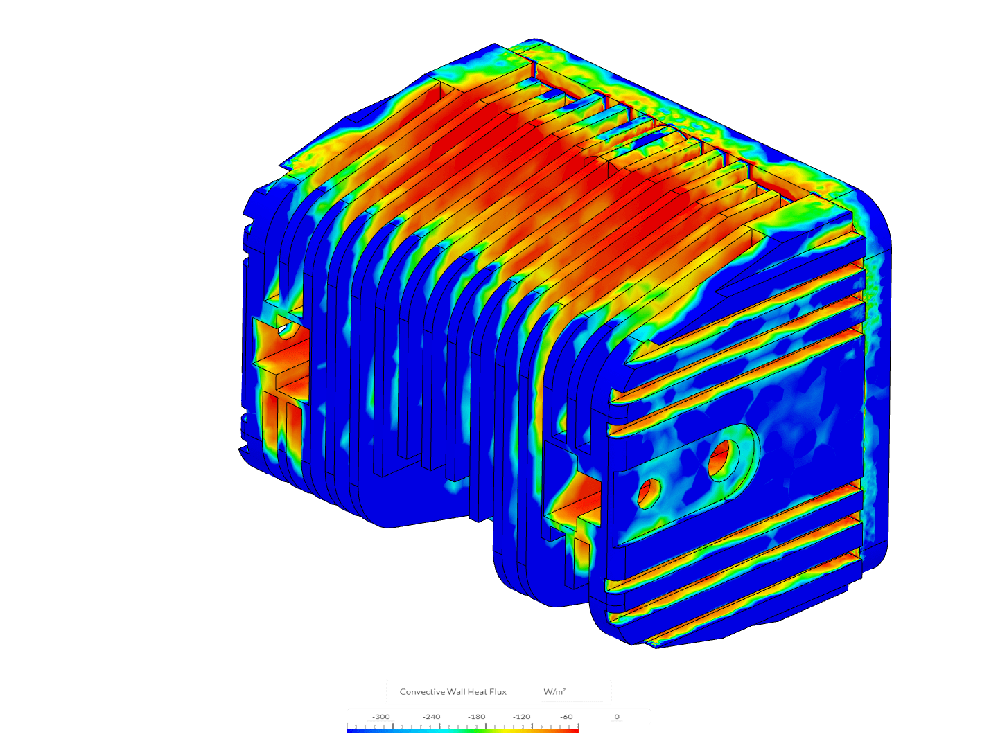
Heat flux can be viewed as a global result quantity as well as with filters such as isovolumes. The image below shows a high-powered LED light that has a heat sink included in the housing frame. The areas of blue represent high levels of heat flux from the heat sink & housing, therefore implying a high-performing area. It is clear that a lot of the heat is rejected at the end of the heat sink fins, out where there is access to ambient, cool air.
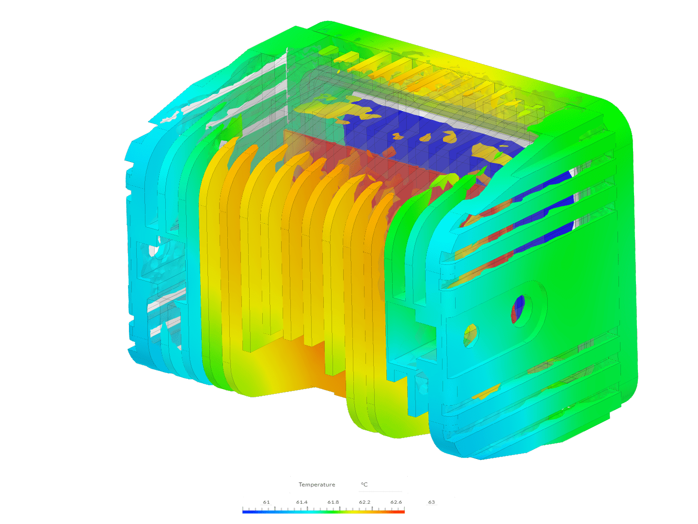
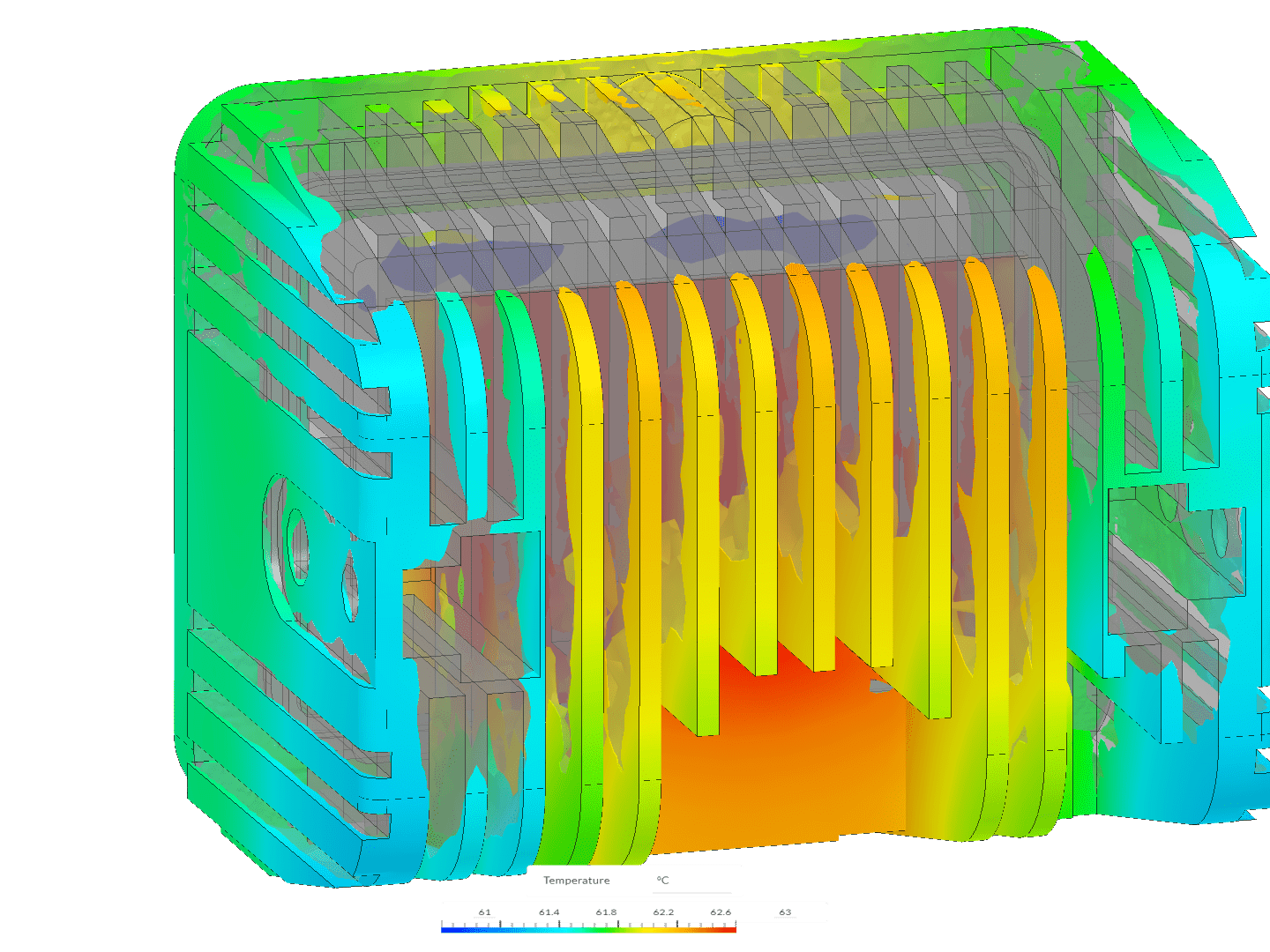
Furthermore, we can use isovolumes to identify areas of high thermal flux. For example, the image below uses an isovolume to show areas with a heat flux of -100 \(W/m^2\) and less.
Last updated: March 16th, 2026
Did this article solve your issue?
How can we do better?
We appreciate and value your feedback.
What's Next
Numerics Background for CFD and FEA

