Mathematical Fundamentals - Gradient, Gauss' divergence theorem and Green-Gauss theorem

[jousefm]

Introduction

I showed in Chapter 5 of the FEM fundamentals how to obtain the weak form from the strong form. The integration by parts was necessary!

In 2D or 3D, a similar integration type needs to be used. For this purpose we will make use of the Green-Gauss theorem, which is based on the Gauss divergence theorem.

Before talking about these theorems, we discuss the concept of the gradient.

---

The Gradient

The term gradient has different meanings in mathematics. One of the most common associations with gradient is the slope.

The gradient as I will explain it, is often denoted by the symbol \nabla (“Nabla”) and is often applied to a real function of three variables f(x_1,x_2,x_3) and can also be written as:

\nabla f \equiv grad(f)

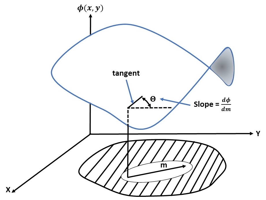
Consider a two-dimensional quantity \phi which is dependent from two variables (x,y), i.e. \phi = \phi(x,y). If we want to know how \phi varies over the region in which its variables x and y are defined, we use the chain rule and get:

d\phi = \frac{\partial\phi}{\partial x} dx + \frac{\partial\phi}{\partial y} dy \tag{1}

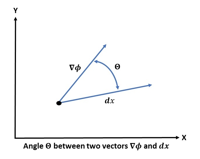
The meaning of expression (1) is illustrated in the following graphic:

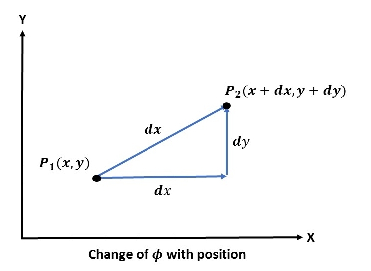
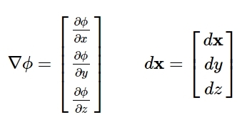
We will now introduce the column matrices \nabla \phi and d\mathbf{x}:

From the figure above d\mathbf{x} appears to be a vector with the components dx and dy. We can consider the same for the column matrix \nabla \phi with the components \partial\phi/\partial x and \partial\phi/\partial y in the x- and y-directions. The vector \nabla\phi is called the gradient of \phi. With the two column matrices above, expression (1) can be written as:

where d\phi is the scalar product of \nabla\phi and d\mathbf{x}.

In general the scalar product is given as:

d\phi = (\nabla\phi)^T d\mathbf{x} = |\nabla\phi| |d\mathbf{x}| cos\theta \tag{3}

where |\nabla\phi| and |d\mathbf{x}| are the lengths of the corresponding vectors and \theta is the angle between those two vectors.

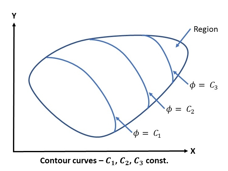
Contour curves can be identified along which our quantity \phi remains constant, as \phi = \phi(x,y). We can achieve this if we set \phi(x,y) = C, where C is a constant. It follows that this expression provides us with a relation between x and y and describes a so called contour curve:

If we move along the contour curves, \phi is constant and we can assume that there is a vector d\mathbf{x} which is directed tangentially to this curve:

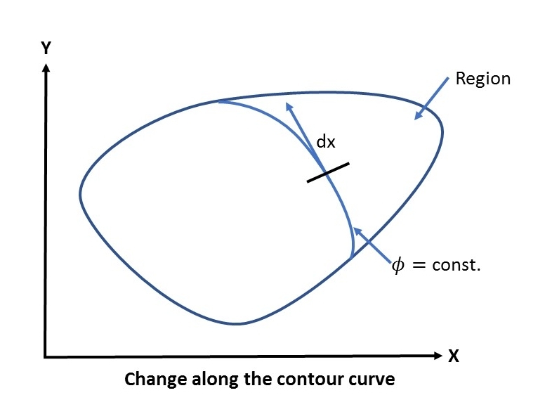
As \phi is constant along the curve we can conclude from equation (3) that:

d\phi = (\nabla\phi)^T d\mathbf{x} = |\nabla\phi| |d\mathbf{x}| cos \theta = 0

which can only be fulfilled if cos\theta = 0. That means that the two vectors are orthogonal. Since d\mathbf{x} is orthogonal to the contour curve, we also know that the gradient \nabla\phi is orthogonal to the contour curve.

Another interesting question is in which direction \nabla\phi is showing. For this purpose we shall look at two infinitely close contour curves:

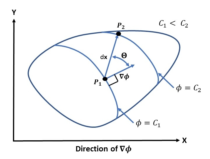
If we move from point P_1 to P_2 along d\mathbf{x} we can see that \phi is larger at the second point (P_2) than in P_1. With expression (3) we can conclude that the expression has to be larger than 0:

d\phi = (\nabla\phi)^T d\mathbf{x} = |\nabla\phi| |d\mathbf{x}| cos \theta > 0

This is only true if the cos\theta > 0, which means that \nabla\phi is directed in the direction of increasing values of \phi as indicated in the picture above.

\boxed{\text{The gradient $\nabla\phi$ is orthogonal to the contour curve}} \qquad \text{and} \qquad \boxed{\text{The direction of $\nabla\phi$ is in the direction of the increasing $\phi$-values}}

We can also conclude from equaton (3) that the largest increase of \phi only is possible when d\mathbf{x} is in the direction of the gradient itself.

Expression (3) can be rewritten in a more convenient way. The length of d\mathbf{x} can be substitude by dm:

dm = |d\mathbf{x}| = (dx^2+dy^2)^\frac{1}{2} \tag{4}

We can then define a unit vector m in the direction of d\mathbf{x}. Splitting the components of m in m_x and m_y we get:

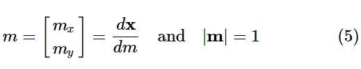
If we now divide expression (3) by dm and use the equation (5), it follows that:

\boxed{\frac{d\phi}{dm} = (\nabla\phi)^T\mathbf{m}} \tag{6}

We can observe that the fraction d\phi/dm is the slope of \phi in the direction of the derived unit vector m:

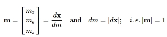
The whole derivation of the gradient can also be done for three dimensions \phi = \phi(x,y,z). The gradient \nabla\phi and d\mathbf{x} are given by:

and the unit vector m:

Gauss’ divergence & Green-Gauss theorem

Mathematical proofs of the now heurisitc derived theorems can be found in Kaplan(1981), Kreysig(1979) and Sokolnikoff and Redheffer (1958).

For the function \phi = \phi(x,y) defined over the area A (shown in the illustration below), consider an area integral

\int_A \frac{\partial \phi}{\partial x} dA \tag{7}

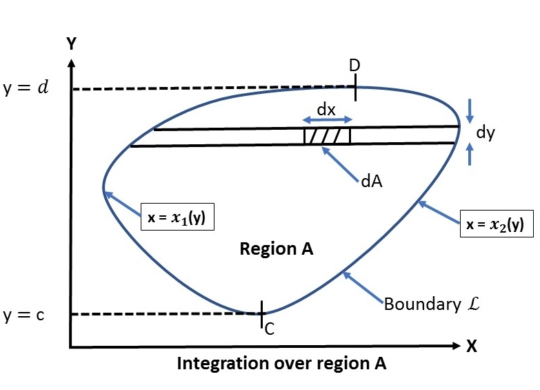
In the picture, points C and D indicate the maximum and minimum y-values. These two points divide the region into two curves x=x_1(y) & x=x_2(y).

Evaluating the integral given in expression (7), we get:

Expression (8) can be rewritten in a reduced manner since the first term on the right-hand side of the last line is the integral of the curve along the boundary x=x_2(y) and the second term on the right-hand side is the integral of the curve along the boundary x=x_1(y), both in couter-clockwise direction.

\int_A \frac{\partial \phi}{\partial x}dA = \oint_\mathcal{L} \phi(x,y) dy \tag{9}

Formula (9) can be rewritten by using an incremental arc length d\mathcal{L} along the boundary. For this purpose consider the following image:

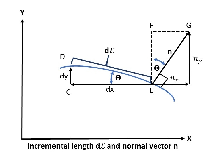
The normal vector n can be written as a column vector with n_x and a n_y component. Its length is given by:

|\mathbf{n}| = (n_x^{2} + n_y^{2})^\frac{1}{2} = 1 \tag{10}

The incremental vector d\mathcal{L} is given by:

\boxed{d\mathcal{L} = (dx^2 + dy^2)^\frac{1}{2}} \tag{11}

According to the illustration above, the angle \theta can be identified two times. The first time in the triangle EFG and the second time in the triangle ECD:

cos\theta = \frac{CE}{ED} = \frac{FE}{EG}; \qquad sin\theta = \frac{CD}{ED} = \frac{FG}{EG}

Putting in the lengths:

-\frac{dx}{d\mathcal{L}} = \frac{dy}{d\mathcal{L}} = \frac{d_x}{1}

where CE = |dx| = -dx

\implies dx = - n_y d\mathcal{L}; \qquad dy = n_x d\mathcal{L} \tag{12}

Using equation (9) and (12) we get:

\int_A \frac{\partial \phi}{\partial x}dA = \oint_\mathcal{L} \phi n_x d\mathcal{L} \tag{13}

The same goes with an arbitrary function \psi:

\int_A \frac{\partial \psi}{\partial y}dA = \oint_\mathcal{L} \psi n_y d\mathcal{L} \tag{14}

We introduce another arbitrary component, the so called vector \mathbf{q}:

\mathbf{q} = [\phi \quad \psi]^T \tag{15}

Adding (13) & (14) with the use of (15), we obtain:

\boxed{\int_A div \ \mathbf{q} \ dA = \oint_\mathcal{L} \mathbf{q}^T \mathbf{n} \ d\mathcal{L}} \tag{16}

where div \ \mathbf{q} is the divergence of \mathbf{q} defined by

\boxed{div \ \mathbf{q} = \frac{\partial q_x}{\partial x} + \frac{\partial q_y}{\partial y}} \tag{17}

Considering a vector \phi\mathbf{q} instead of \mathbf{q} where \phi is a scalar, we now use expression (17):

div(\phi \mathbf{q}) = \frac{\partial}{\partial x}(\phi q_x) + \frac{\partial}{\partial y}(\phi q_y) = \phi \frac{\partial q_x}{\partial x} + \phi \frac{\partial q_y}{\partial y} + \frac{\partial \phi}{\partial x} q_x + \frac{\partial \phi}{\partial y} q_y \tag{18}

Using the definition of the gradient \nabla \phi we get:

div(\phi \mathbf{q}) = \phi \ div \ \mathbf{q} + (\nabla \phi)^T \mathbf{q} \tag{19}

Inserting \phi \mathbf{q} instead of \mathbf{q} into (16) and use (19), we get the Green-Gauss theorem:

\boxed{\int_A \phi \ div \ \mathbf{q} \ dA = \oint_\mathcal{L} \phi\mathbf{q}^T\mathbf{n} \ d\mathcal{L} - \int_A (\nabla \phi)^T \mathbf{q} \ dA} \tag{20}

This Green-Gauss theorem can be seen as the 2D counterpart for integration by parts.

There are some different notations for this theorem. If the arbitrary vector \mathbf{q} is chosen so that q_x = \psi and q_y = 0 the equation becomes:

\boxed{\int_A \phi \frac{\partial \psi}{\partial x} dA = \oint_\mathcal{L} \phi \psi n_x \ d\mathcal{L} - \int_A \frac{\partial \phi}{\partial x}\psi \ dA} \tag{21}

If \mathbf{q} is chosen in a manner so that q_x = 0 and q_y = \psi

\boxed{\int_A \phi \frac{\partial \psi}{\partial y} dA = \oint_\mathcal{L} \phi \psi n_y \ d\mathcal{L} - \int_A \frac{\partial \phi}{\partial y}\psi \ dA} \tag{22}

The whole procedure also works for 3D!

Gauss’ divergence then reads:

\boxed{\int_A div \ \mathbf{q} \ dV = \oint_S \mathbf{q}^T \mathbf{n} \ dS} \tag{23}

where we now integrate the div(\mathbf{q}) over a volume V and the quantity \mathbf{q}^T\mathbf{n} is integrated over the surface. The final form looks like this:

\boxed{\int_A \phi \ div \ \mathbf{q} \ dV = \oint_S \phi\mathbf{q}^T\mathbf{n} \ dS - \int_V (\nabla \phi)^T \mathbf{q} \ dV} \tag{24}

Hints:

In CFD this Gauss theorem is used to get the basic FVM formulation from a flux integral.

Note: Transforming the volume to a surface integral brings you back to the form used for the derivation of the Navier–Stokes equations.

Applications of the mathematical derived theorems and how they are used in CFD (Open$\nabla$FOAM):

Click \rightarrow NUMERICAL SCHEMES

---

Sources:
• Introduction to the Finite Element Method - Niels Ottosen & Hans Petersson
• Gradient - Wikipedia
• Gradient -- from Wolfram MathWorld
• Divergence theorem - Wikipedia
• Green's theorem - Wikipedia

Pictures:
Created with PowerPoint2016

Errata:
If you find mistakes, please do not hesitate to contact me.