The Courant–Friedrichs–Lewy or CFL condition is a condition for the stability of unstable numerical methods that model convection or wave phenomena. As such, it plays an important role in computational fluid dynamics (CFD).
The section below confers the numerical discussion that derives the CFL condition. After this discussion, the CFL condition is presented, and in later sections, its practical consequences are examined.
CFL Condition What is the CFL Condition?
Culbert B. Laney’s definition of the CFL condition, from the book “Computational Gasdynamics”, is as follows: the full numerical domain of dependence must contain the physical domain of dependence.
Therefore, the CFL condition expresses that the distance that any information travels during the timestep length within the mesh must be lower than the distance between mesh elements. In other words, information from a given cell or mesh element must propagate only to its immediate neighbors.
The CFL condition is commonly confused with linear stability conditions or nonlinear stability conditions. However, it’s important to emphasize that it is not a sufficient condition for stability, and other stability conditions are generally more restrictive than the CFL condition.
CFL Derivation
We can derive the CFL condition in a simple and intuitive way. Let’s begin by considering the simple linear convection problem of a quantity u:
$$ \frac{\partial u}{\partial t} + a \frac{\partial u}{\partial x} = 0 $$
For the simple problem of linear convection of a quantity u, the first-order explicit upwind scheme becomes:
$$ \frac{u_i^{n+1} – u_i^n}{\Delta t} + \frac{a}{\Delta x} \left(u_i^n – u_{i-1}^n \right) = 0 $$
where a is the velocity magnitude, Δt is the timestep, and Δx is the length between mesh elements.
By performing a Taylor series expansion on this scheme, this scheme introduces what is called a numerical diffusion, or numerical viscosity, equal to:
$$ \mu_{num} = a \frac{\Delta x}{\Delta 2} \left(1- \frac{a \Delta t}{\Delta x}\right) $$
As expected from a diffusion coefficient, the numerical diffusion coefficient must be positive, otherwise, the solution will grow indefinitely with respect to time, making the numerical scheme unstable.
The right term inside the parenthesis of the above expression is commonly referred to as the Courant number, which is a dimensionless quantity. Therefore, the Courant number can be stated as follows:
$$ C = a \frac{\Delta t}{\Delta x} $$
It follows from the numerical diffusion coefficient discussion, that for any explicit simple linear convection problem, the Courant number must be equal or smaller than 1, otherwise, the numerical viscosity would be negative:
$$ C \le 1 $$
An article by Courant, Friedrichs, and Lewy first introduced this condition in 1928. This derivation is considered to be one of the most influential works for the development of CFD techniques.
CFL Problems Other Types of Problems for the CFL Condition
This discussion may only hold true for explicit schemes. It is important to also briefly discuss what occurs in more realistic problems.
Firstly, implicit linear convection is unconditionally stable and also lacks a CFL condition. This happens because implicit schemes use the entire domain to calculate each timestep. However, implicitly calculating (i.e., solving an implicit linear system) each timestep can be very costly. In addition, time accuracy decreases as the timestep increases. Therefore, it is logical to use an explicit scheme with a lower timestep.
For more complicated and representative problems, including nonlinear flow, the CFL condition serves as a reference for setting the timestep. Furthermore, when dealing with nonlinear phenomena, even the implicit form can have stability problems if a large Courant number is chosen. Consequently, it might be necessary to apply local stability analysis on a linearized formulation in those cases. Still, the CFL condition is necessary for nonlinear problems.
Common CFL Usage
The best way to understand how the CFL number is used is to try to put it into practice. Here is a simulation that can be used as a template for your own project. All you need to do is create a free Community account here, copy the project, and start simulating. To learn more about cloud-based CFD simulation with SimScale, check out the CFD product page below.
Explore CFD in SimScale
Let’s begin by understanding the problem being simulated.
Knowing the Problem
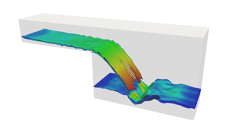
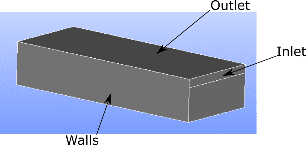
The problem geometry is intentionally simple. It consists of a rectangular box with an inlet and an outlet. From the inlet, we will prescribe a velocity inlet boundary condition for a fluid such as water, and the outlet will consist of a prescribed pressure boundary condition.
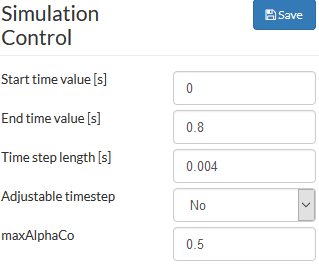
Keeping the problem simple allows experimentation with the Courant number so we can visualize the consequences. The interest lies in what occurs when the timestep value is increased. The timestep can be adjusted on the Simulation Control panel:
Finding Your Courant Number
The adjustable timestep option has been purposely disabled to avoid simulation back-end interference. If this option is activated, the solver would do its best to converge the simulation, as that’s what is generally preferred.
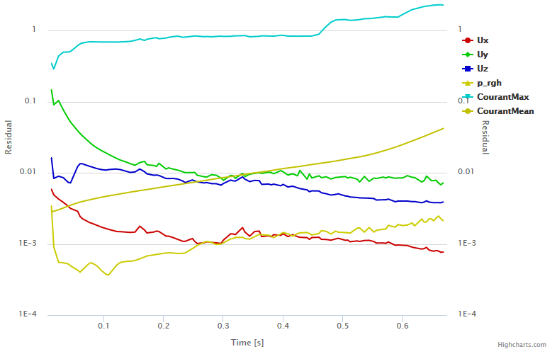
To start building experiments, choose a timestep of 0.001 seconds for an inlet velocity of 5m/s. The convergence plot is as follows:
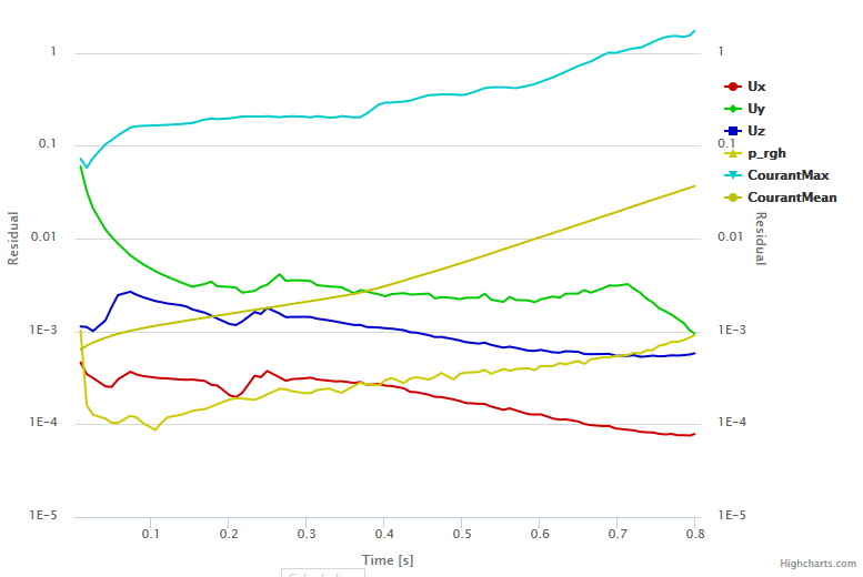
On inspection of the plot, it’s clear that eventually, the maximum Courant value for the problem exceeds the value 1. Within the program, SimScale displays a warning informing that this can cause high instability in the simulation. However, the simulation still converges in this case. It’s important to notice, however, that the simulation result will probably be unreliable under such conditions.
By increasing the timestep to just 0.004 seconds, the Courant number goes above 2.0, causing the solver to diverge and display an error. The simulation is then interrupted:
Solving CFL Convergence Problems
There are several ways to solve such convergence problems. Recall the Courant number:
$$ C = a \frac{\Delta t}{\Delta x} $$
To lower this value, one can:
- Lower the timestep, or
- Make a coarser mesh.
The second option is sometimes counterintuitive for some since it doesn’t seem rational that a coarser mesh can help convergence. However, it is quite understandable that a finer mesh helps accuracy. This motivates engineers to create finer meshes, but forget to reduce the timestep value.
Regarding the first option, the correct timestep value is not always obvious. The problem can have complex phenomena that occur during the simulation. This requires the engineer to set a low timestep for the simulation, even if these complex phenomena only happen in a small fraction of the simulation time.
SimScale’s backend solver allows for the use of an adjustable timestep. This option is activated by default, and has two parameters:
- Maximum Courant number, and
- Maximum timestep
Set the Maximum Courant number to a safe value, such as 0.5, and see what happens to the simulation:
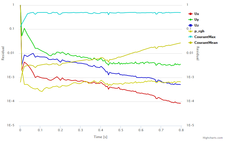
The solver was able to keep the maximum Courant number around 0.5, which was enough for the simulation to converge nicely.