Tutorial: Nonlinear Structural Analysis of a Wheel

This article provides a step-by-step tutorial for the nonlinear structural analysis of a wheel. The objective of this simulation is to analyze the deformation and stress distribution across the wheel in operation mode, taking into account the nonlinear phenomena such as hyperelastic material, physical contact, and alternating load.

This tutorial teaches how to:

• Set up and run a nonlinear structural analysis.
• Assign boundary conditions, materials, and other models to the simulation.
• Mesh the geometry with SimScale’s standard meshing algorithm.
• Explore the results using SimScale’s online post-processor.

The typical SimScale workflow will be followed:

1. Prepare the CAD model for the simulation.
2. Set up the simulation.
3. Create the mesh.
4. Run the simulation.
5. Analyze the results.

1. Prepare the CAD Model and Select Analysis Type

To start, you can import a copy of the project into your workbench by following along the steps by clicking the button below:

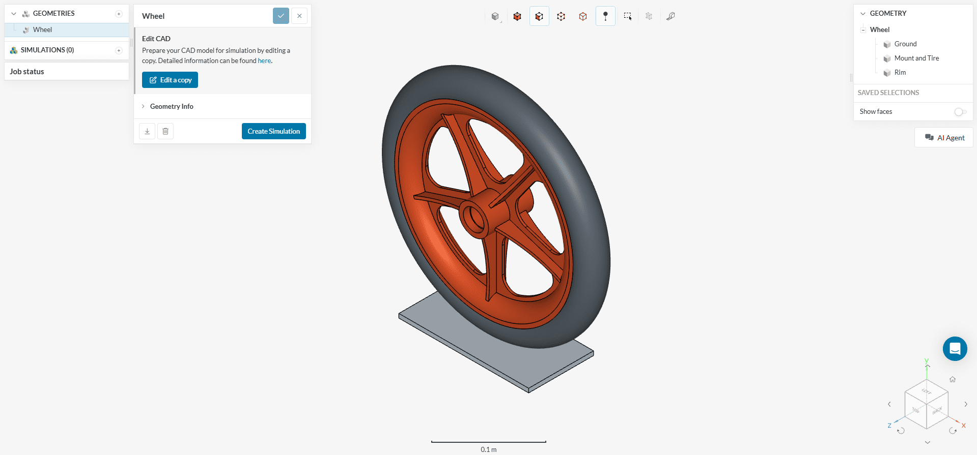
The image below illustrates the view after importing the tutorial project. The geometry Wheel appears in the simulation tree, and its corresponding 3D model is displayed in the Workbench. The model can be explored interactively—rotate, zoom, and pan using standard CAD navigation controls.

This simulation takes advantage of the model’s double symmetry for two main purposes:

• Reduce computational cost by simulating only a portion of the full geometry
• Prevent rigid body motion in the X and Y directions, enhancing numerical stability

Utilizing symmetry whenever possible is recommended, as it leads to faster and more stable simulations without compromising accuracy.

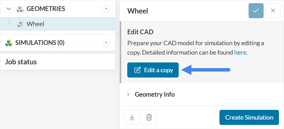
The ‘Edit a Copy’ option in the geometry pop‑up (Figure 3) launches the CAD Edit environment. Within this workspace, the ‘Split’ operation isolates the symmetrical portion of the model, removing redundant geometry and retaining only the region required for the simulation.

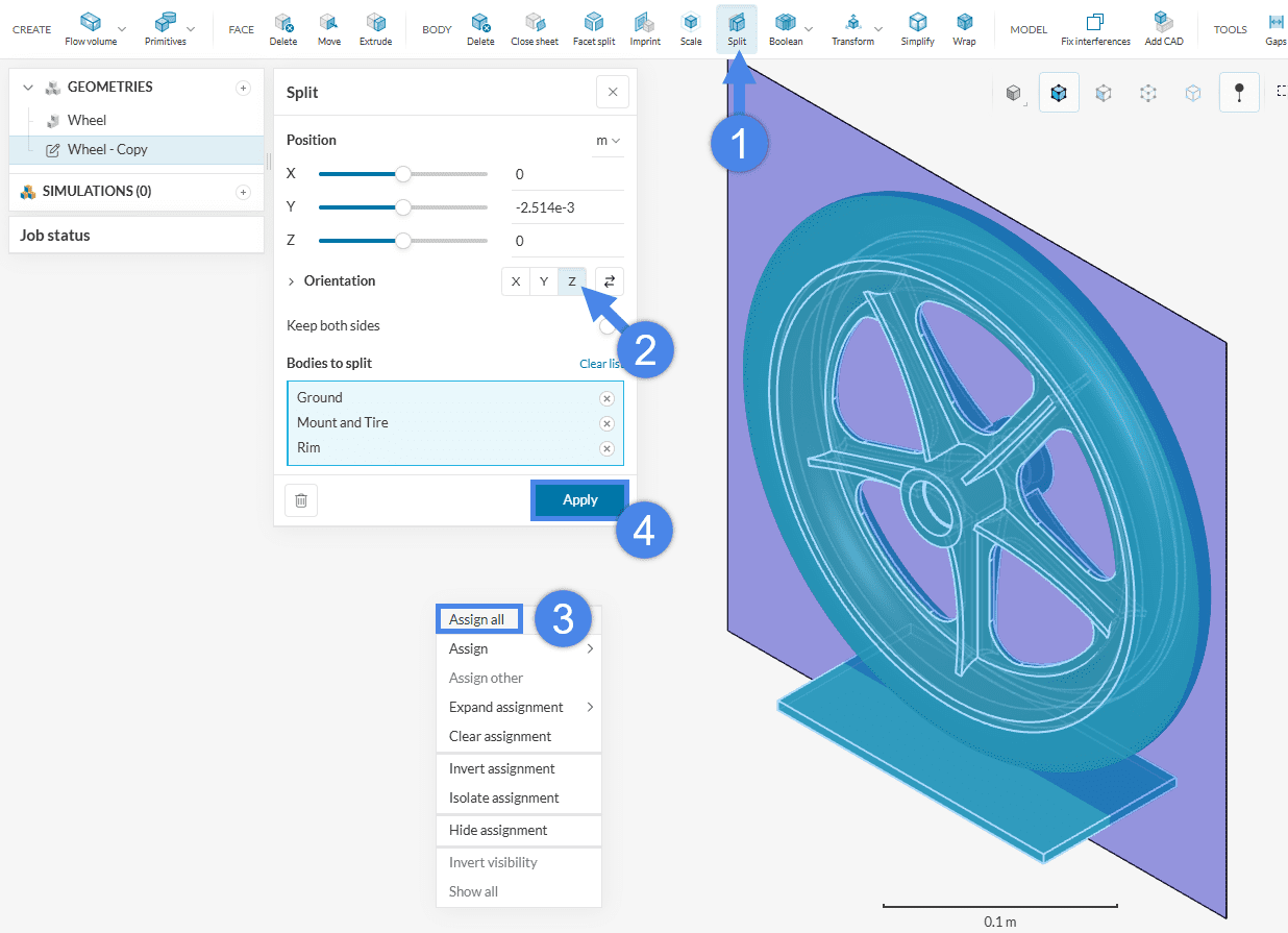
1. Select the ‘Split’ operation from the toolbar in the CAD Edit environment.
2. Set the orientation to ‘Z’.
3. Right click anywhere in the Workbench and click ‘Assign all’
4. Select the bodies to be split and click ‘Apply’.

This operation extracts one half of the model.

To obtain the quarter symmetry, repeat the ‘Split’ operation:

• Change the orientation from ‘Z’ to ‘X’
• Use the button highlighted in Step 3 of Figure 5 to align the cutting plane with the ‘–X’ direction

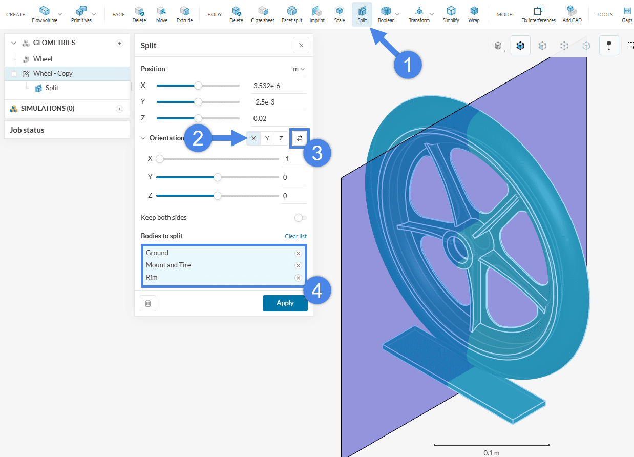
The resulting geometry should resemble the one shown below, representing one-quarter of the original model aligned with both symmetry planes. This reduced model retains the essential structural behavior while significantly decreasing computational effort.

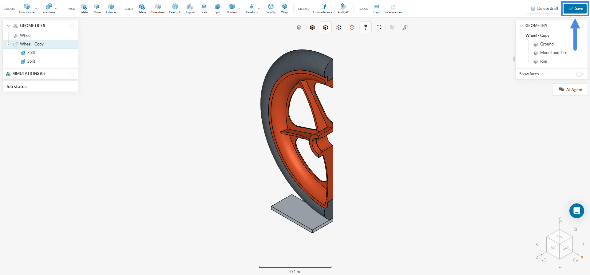
Finally, click ‘Save’ in the top-right corner to apply the changes and import the modified geometry into the Workbench for simulation.

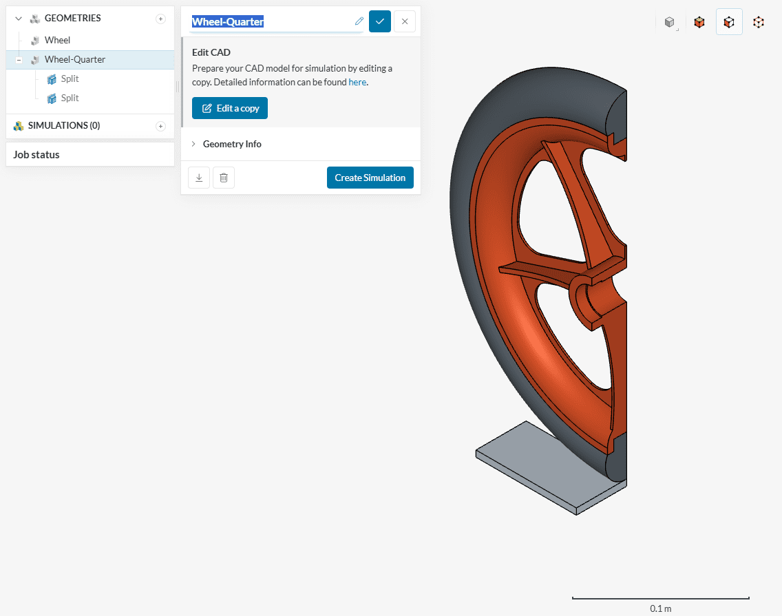
The newly created geometry will appear as ‘Copy of Wheel’ by default. Rename it to something more descriptive, such as ‘Wheel–Quarter’, for easier identification during the simulation setup.

1.1 Create a Nonlinear Structural Analysis

Now the simulation setup can be started. Follow these steps to create a new simulation:

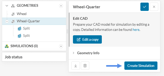
1. Select the ‘Wheel-Quarter’ geometry in the left panel.
2. Click the ‘Create Simulation’ button in the pop-up window.

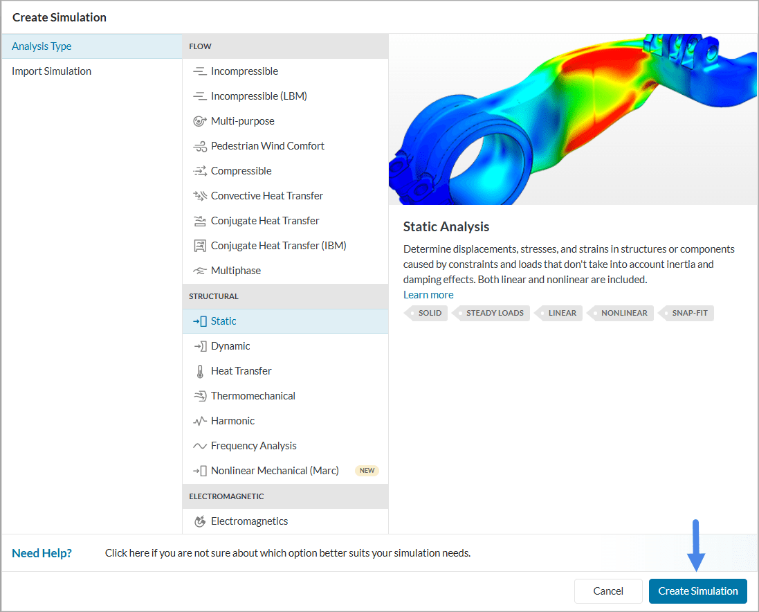
The simulation library window appears. Select the ‘Static’ analysis type and click the blue ‘Create Simulation’ button at the bottom:

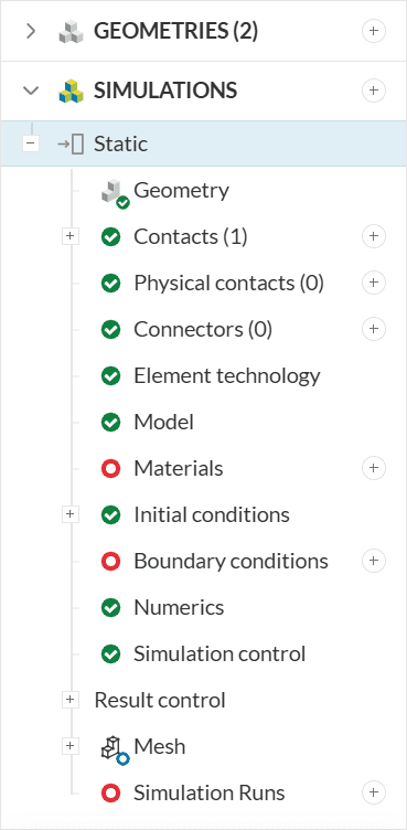
A new simulation tree is then automatically generated in the left panel, containing all the parameters and settings required to fully define the analysis. Each item in the tree is marked with a status indicator: a green check signifies that the item is complete, a red circle indicates a required input that is still missing, and a blue circle denotes an optional setting. These visual cues help guide the simulation setup process. Refer to the figure below for an illustration.

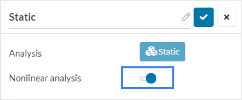
Since this structural simulation involves nonlinearities—such as physical contact, hyperelastic material behavior, and varying loads—the nonlinear analysis option must be enabled. In the ‘Global settings’ panel that appears after creating the simulation, activate the ‘Nonlinear analysis’ toggle to account for these effects in the solver.

You can find more details about what characterizes a static analysis here.

2. Set Up the Nonlinear Structural Analysis

The analysis of the wheel will include the following operating conditions:

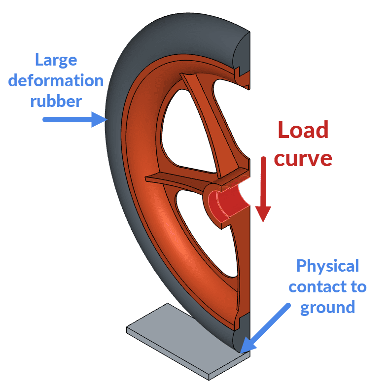
In this simulation, the wheel rim is modeled using polypropylene, a common thermoplastic material. The wheel tire is defined as rubber, a hyperelastic material expected to undergo large deformations under load.

The loading conditions include:

• A maximum operating load of 1000 \(N\)
• A mean operating load of 500 \(N\)

To realistically capture the interaction between the tire and the ground, the model must include physical contact between these two components.

The figure below summarizes the key nonlinear modeling conditions applied in this analysis.

2.1 Contacts

Two contact conditions are defined in this simulation:

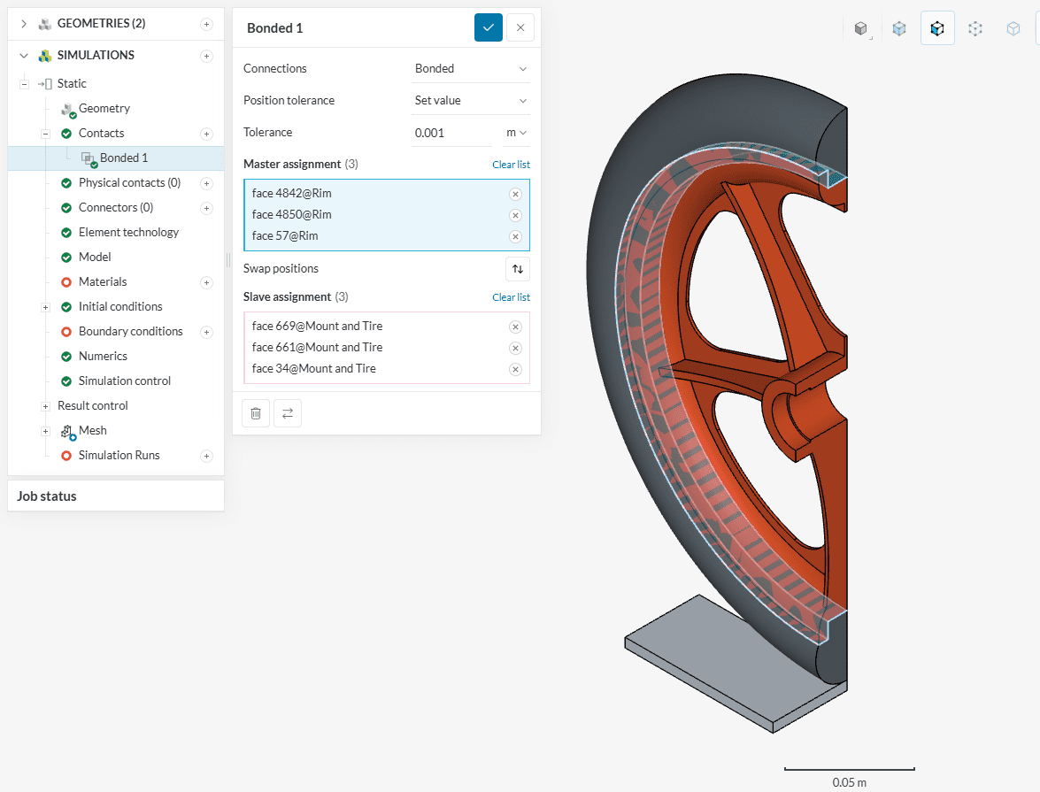
• Rim–tire interface: A linear bonded contact is specified to ensure compliant deformation between the rim and tire.
• Tire–ground interface: A nonlinear physical contact is specified to capture realistic interaction behavior, including separation and compression.

The bonded contact between the rim and tire is automatically detected and created by SimScale. It appears under the ‘Contacts’ section in the simulation tree as Bonded 1.

Next, create a Physical contact definition to define the interaction between the tire and the ground. Follow the steps illustrated in the accompanying image to assign the correct surfaces and parameters. This contact setup enables the solver to accurately model the nonlinear deformation and contact response under load.

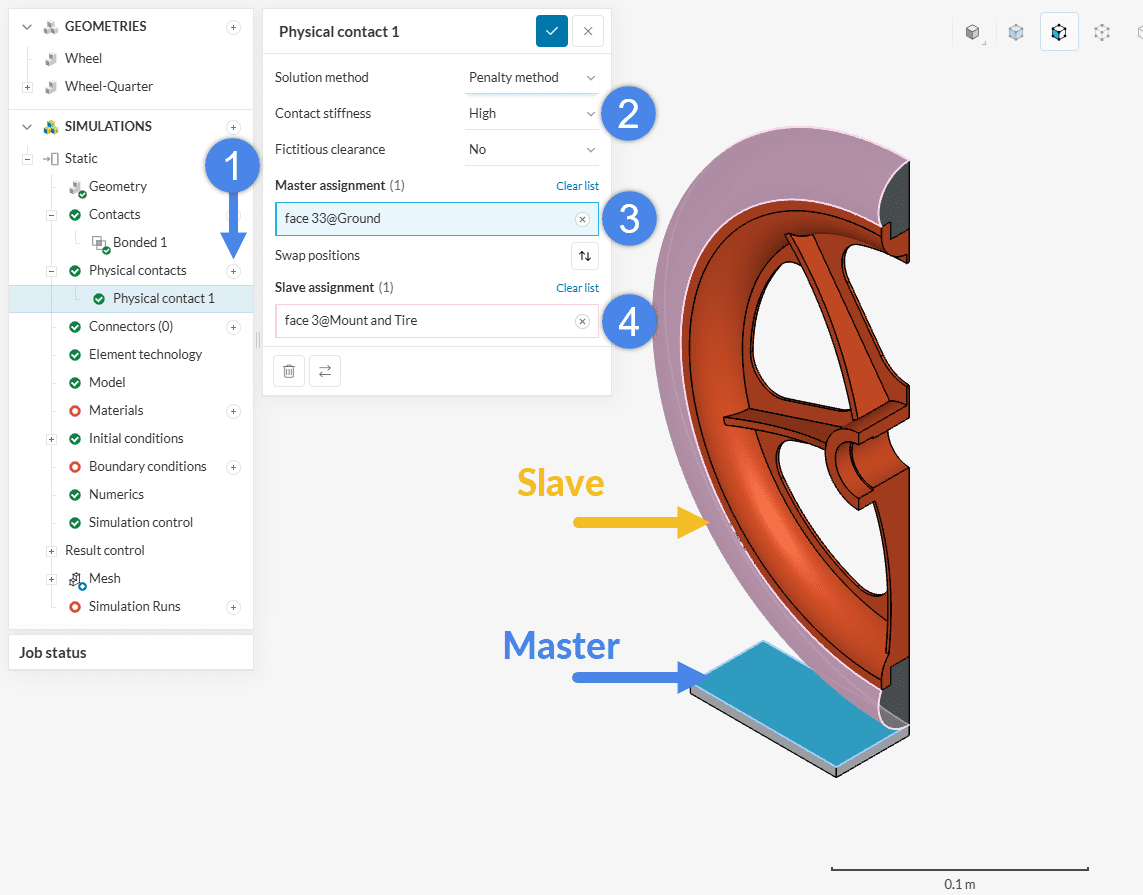
1. Click the ‘+’ icon next to Physical contacts and select ‘Physical contact’ from the menu.
2. Change the Contact stiffness to ‘High’.
3. Click on the Master assignment box, then select the corresponding face from the ground part.
4. Click on the Slave assignment box, then select the corresponding face from the tire.

Click the check mark to finish the setup.

The selection of faces to be assigned the master/slave is performed according to the key concepts explained in the following article.

Which Surface Should I Select as the Master in a Contact Pair?

2.2 Material Model

To define the material behavior, add the required material models from the material library. Begin by clicking the ‘+’ button next to the Materials node in the simulation tree. This opens the materials library, where the appropriate material can be selected. After selecting the desired material, click ‘Apply’ to load its standard properties into the simulation setup.

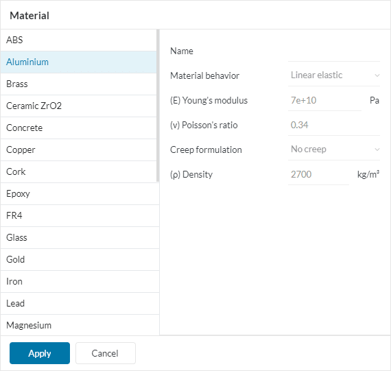
In the settings panel, the target body that will have the material properties applied is assigned. Accept the selection with the blue checkmark .

Use these instructions to assign the following material to each body in the CAD model:

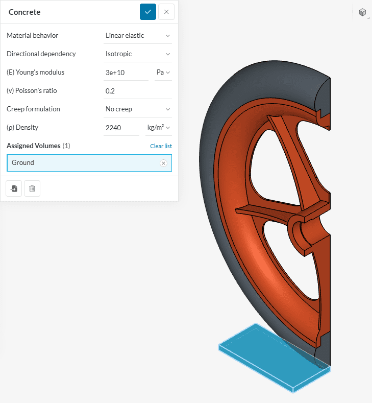
A. Ground

For the ground body, select Concrete from the material library. Assign it to the Ground geometry by selecting the corresponding body either directly in the viewer or from the Scene tree on the right panel, as illustrated in the figure below.

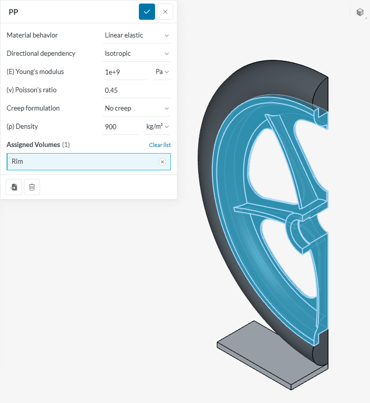
B. Rim

For the wheel rim, select the PP (polypropylene) material from the material library, and assign the Rim body.

C. Tire

For the wheel tire, select Rubber from the material library and assign it to the Mount and Tire bodies. Due to the softness of this component and the expected large deformations from loading and contact with the ground, a hyperelastic material model is required.

To configure this:

• Change the Material behavior setting to ‘Hyperelastic’
• Input the material parameters as shown in the accompanying image

This setup ensures accurate representation of the nonlinear elastic response of the rubber material.

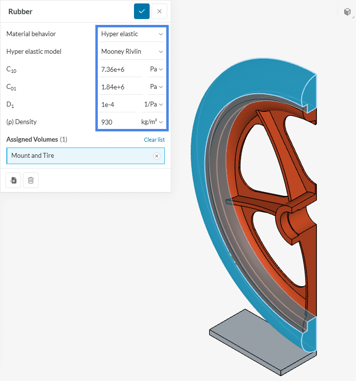
The input values are:

• Hyperelastic model: Mooney-Rivlin
• \(C_{10} = \) 7.36e6 \(Pa\)
• \(C_{01} = \) 1.84e6 \(Pa\)
• \(D_{1} = \) 1e-4 \(1/Pa\)
• \(\rho = \) 930 \(kg/m^3\)

2.3 Boundary Conditions

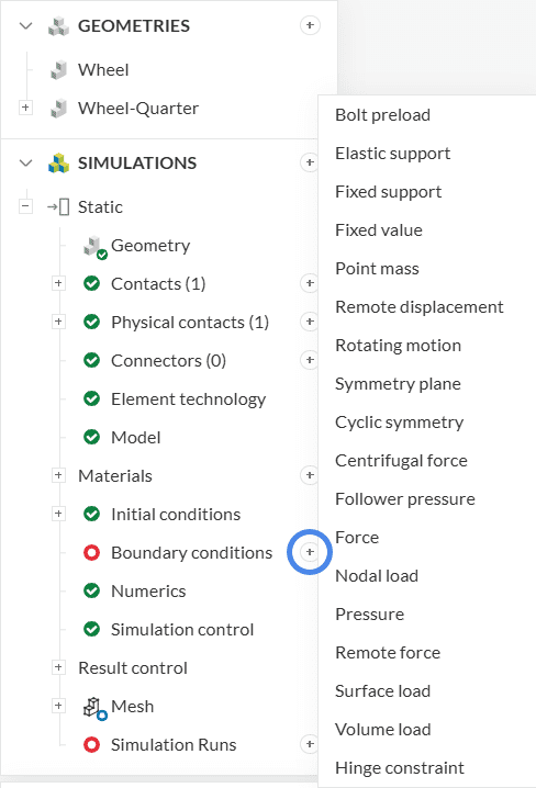
To define the boundary conditions, click the ‘+’ button next to the ‘Boundary conditions’ node in the simulation tree. From the drop-down menu, select the appropriate boundary condition type for the simulation setup, as shown in Figure 19. This step allows the specification of constraints and loads necessary for the analysis.

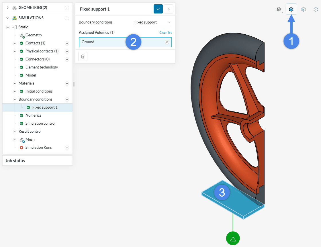
A. Ground Fixed Support

The first boundary condition fixes the ground in place. To define it, select ‘Fixed support’ from the boundary conditions drop-down menu. Then, activate ‘Assign Volume’ from the top toolbar (Figure 20) and select the ground body either in the viewer or from the scene tree. This constraint ensures that the ground remains stationary throughout the simulation.

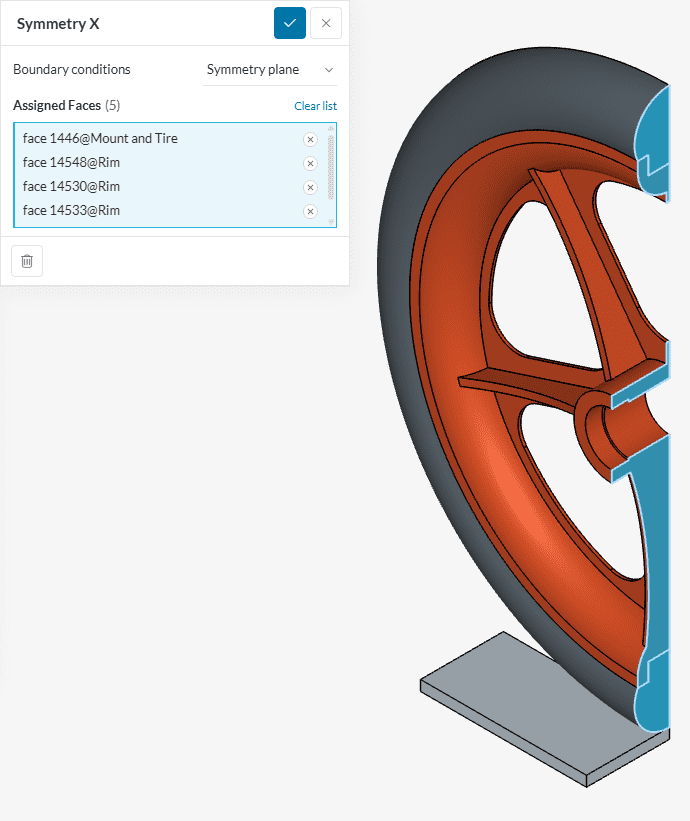
B. Symmetry Plane Normal to X

The second boundary condition restricts normal displacement along the symmetry plane used to cut the model. Select the ‘Symmetry plane’ boundary condition from the list and assign all faces that lie on the symmetry plane, as illustrated in the accompanying image. This constraint ensures that the model behaves as if the full geometry were present.

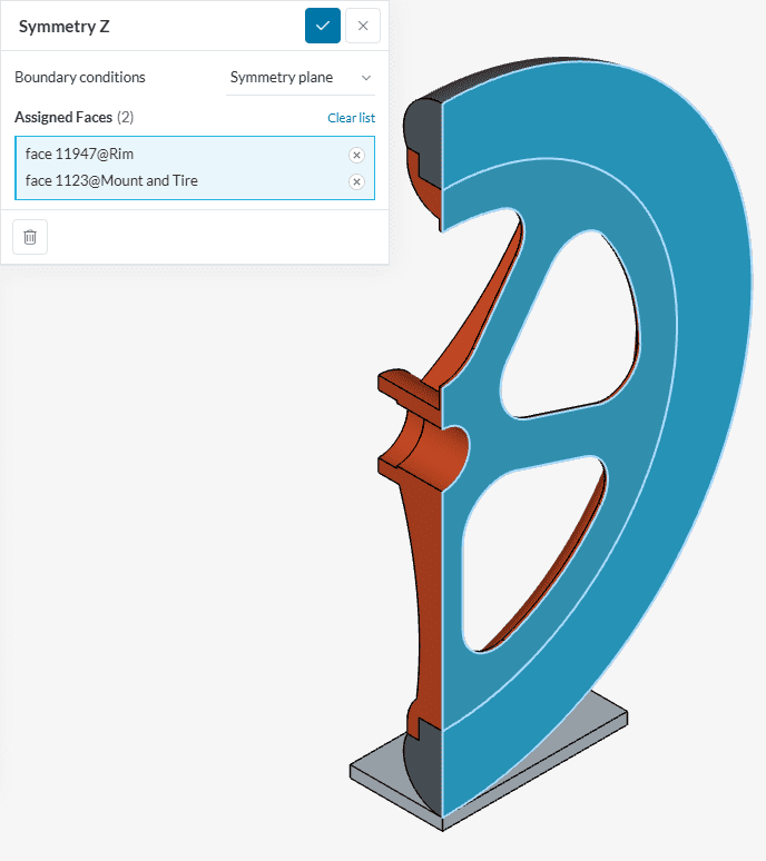
C. Symmetry Plane Normal to Z

Use the same procedure as before to define the second symmetry plane, this time aligned with the ‘Z’ direction. Select the corresponding faces and assign the ‘Symmetry plane’ boundary condition. The process is illustrated in the figure below.

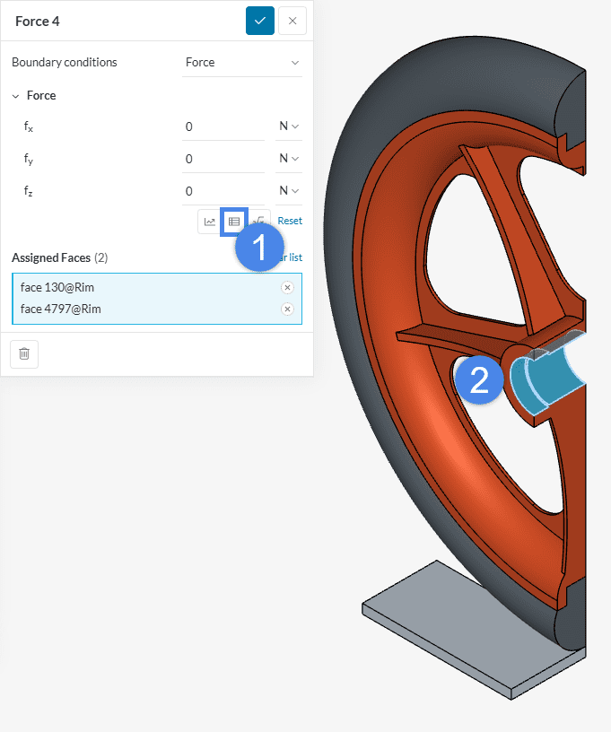
D. Load

To apply the operating load supported by the wheel, select a ‘Force’ boundary condition from the drop-down menu. Click the table icon to define a time-dependent load profile, as illustrated in the accompanying image. Assign it to the central cylindrical faces, as shown in Figure 23.

The Specify value window will appear, allowing input of the load curve. In this case, use the Table input option and configure it as shown in the image below. To visualize the loading profile, change the Column for Y axis to ‘f<y>’. This will generate a graphical representation of the applied force over time.

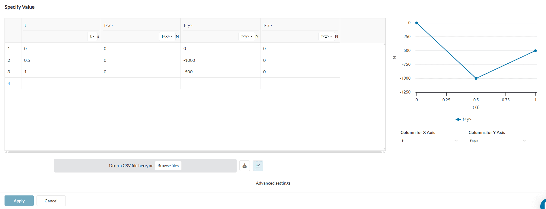
t \([s]\)	Fx \([N]\)	Fy \([N]\)	Fz \([N]\)
0	0	0	0
0.5	0	-1000	0
1.0	0	-500	0

Notice that the load force starts at zero, maxes out at \(t = 0.5\ s\) and then goes back down to the mean value at \(t = 1.0\ s\). The negative value indicates the force direction with respect to the Y axis.

3. Numerics and Simulation Control

The Numerics section of the simulation tree can remain unchanged. The default values are well-calibrated and sufficient for solving this case effectively. In most simulations, modifications to these parameters are unnecessary due to the carefully tuned defaults.

Similarly, no changes are required in the Simulation Control section. Since the simulation interval is assumed to be the default range of 0 to 1, this section can be left as is.

4. Mesh Setup

To achieve optimal results, a structured mesh will be created using the Standard meshing algorithm. Open the Mesh section in the simulation tree and review the default settings, which will remain unchanged. Note that it is not necessary to click ‘Generate’ at this point, as the mesh will be computed automatically during the simulation run.

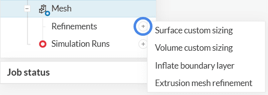
To define mesh refinements and build a structured mesh, click the ‘+’ button next to Refinements under the Mesh node. Then, select the desired refinement type from the available options.

4.1 Extruded Mesh for the Ground

For the first refinement, create an Extrusion mesh refinement. This refinement type enables the generation of structured meshes composed of hexahedral or prismatic elements, which typically offer better numerical performance and accuracy compared to unstructured tetrahedral meshes.

To ensure a valid sweep, select opposite faces that are connected one-to-one at their vertices, as illustrated in the accompanying figure. This ensures proper extrusion and structured element generation across the selected region.

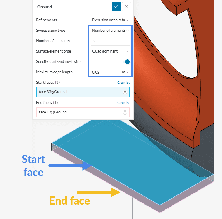
1. Set the Sweep sizing type to ‘Number of elements along sweep’.
2. Set the Number of elements to ‘3’.
3. Set the Surface element type to ‘Quad dominant’.
4. Toggle on the Specify start/end mesh size.
5. Set the Maximum edge length to ‘0.02’ \(m\).
6. Select the Start faces box, then assign the top face of the ground.
7. Select the End faces box, then assign the bottom face of the ground.

4.2 Extruded Mesh for the Tire

The prismatic shape of the tire allows for structured meshing through extrusion. Create a second Extrusion mesh refinement and configure it as shown in the figure. This approach ensures a high-quality mesh for the tire region, improving accuracy in areas expected to undergo large deformations.

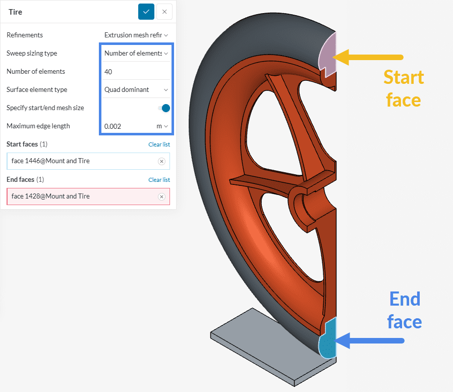
1. Set the Sweep sizing type to ‘Number of elements along sweep’.
2. Set the Number of elements to ’40’.
3. Set the Surface element type to ‘Quad dominant’.
4. Toggle on the Specify start/end mesh size.
5. Set the Maximum edge length to ‘0.002’ \(m\).
6. Select the Start faces box, then assign the shown face.
7. Select the End faces box, then assign the shown face.

4.3 Volume Custom Sizing for the Rim

Finally, since the rim has a more complex geometry that requires an unstructured mesh, apply a Volume custom sizing refinement to control the mesh quality. This refinement limits the element edge length, helping to maintain an optimal aspect ratio and overall mesh resolution.

Create the refinement under Refinements > Volume custom sizing, and configure it according to the parameters shown in the figure.

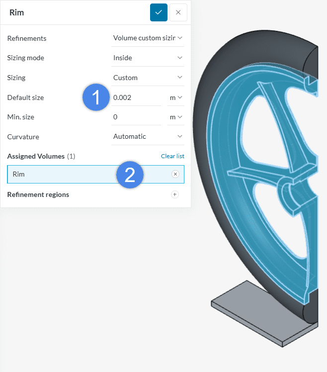
1. Set the Maximum edge length to ‘0.002’ \(m\).
2. Assign the Rim to the refinement.

5. Start the Simulation

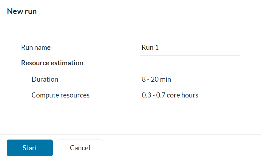
The final step before launching the simulation is to create a run. To do this, click the ‘+’ button next to Simulation Runs in the simulation tree.

In the pop-up window that appears, enter a descriptive name for the run, then click ‘Start’ to begin the computation.

The Job status item below the simulation tree updates the status of the run. Also, a Solver log is provided after a few seconds, which shows the advancements of the actual computing algorithm. The simulation run should take a few minutes to be carried out. Once the simulation run is Finished, we can post-process the results.

6. Post-Processing

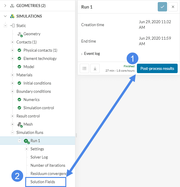
Once the simulation is complete, the wheel load results can be post-processed on the platform using one of the following methods:

• Click on the Completed run entry in the simulation tree, then on Solution Fields to directly access the results
• Use the Post-process results option from the top toolbar to open the results in the post-processor environment

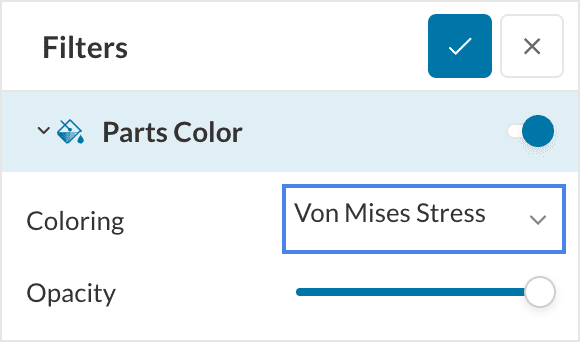
6.1 Visualizing Stress

In order to examine the stress results on the wheel, we should select the field assigned to the Parts Color as ‘Von Mises Stress’:

The parts are now colored according to the levels of stress, but we will perform some tweaking to better visualize the results:

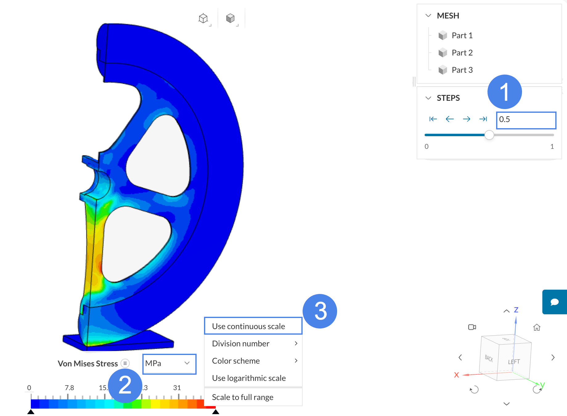
1. Change the time step to ‘0.5’ \(s\), which corresponds to the point of maximum loading.
2. Change the stress units to ‘\(MPa\)’.
3. Right-click on the legend bar and select ‘Use continuous scale’ from the contextual menu.

You should end up with the following visualization:

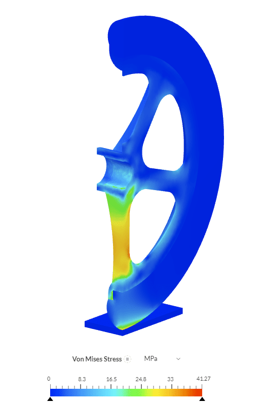
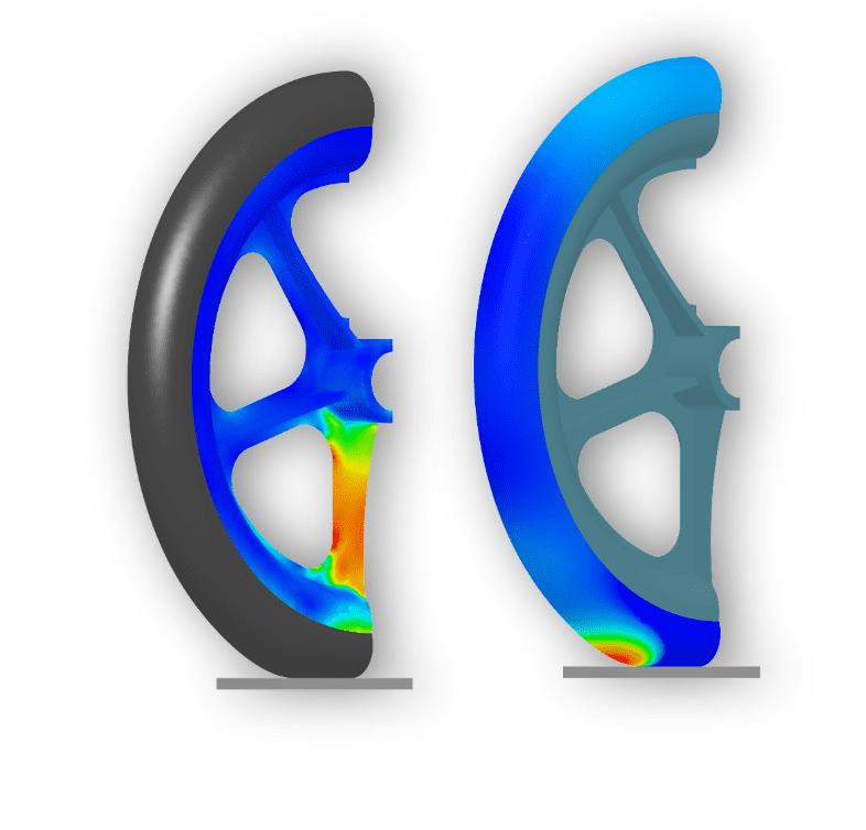
Figure 33 shows the stress distribution on the model of the wheel at the time of maximum load. It can be seen that maximum stress levels of around 41.3 \(MPa\) occur at the rim radius element and at the contact patch between the tire and the ground.

6.2 Deformed Shape

1. In the Parts Color panel, select the ‘Displacement Magnitude’ as Coloring.
2. Right-click on the legend bar and select ‘Use continuous scale’ from the contextual menu.

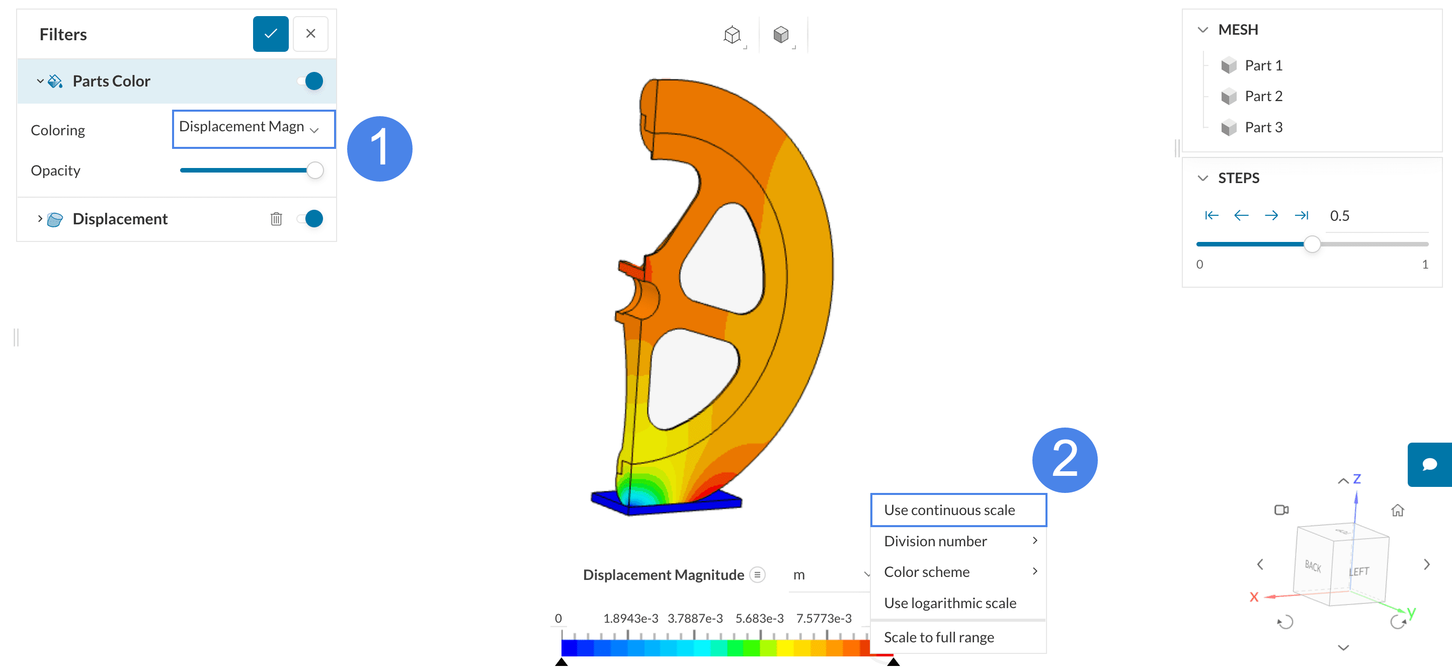
In order to visualize the deformed shape of the wheel, create a Displacement plot:

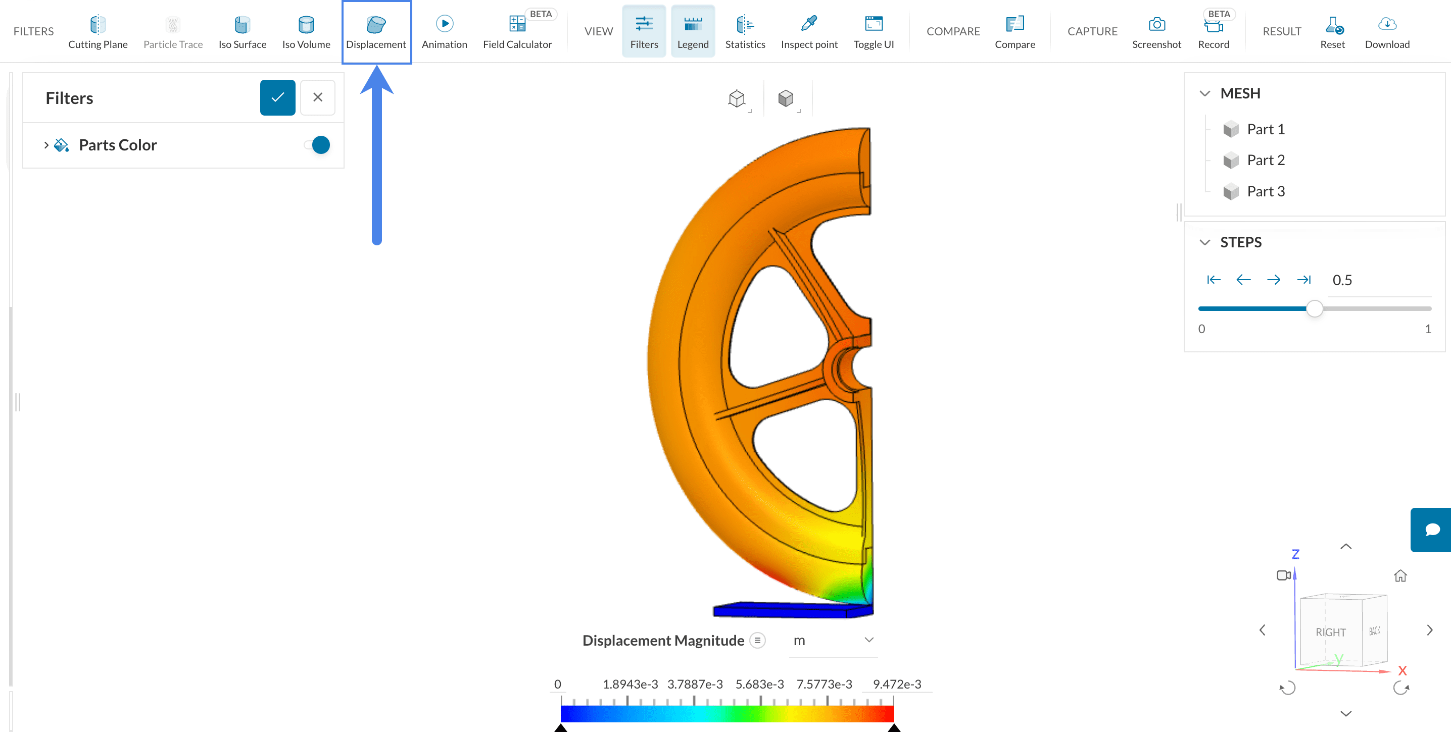
The deformed shape along with the coloring can then be inspected:

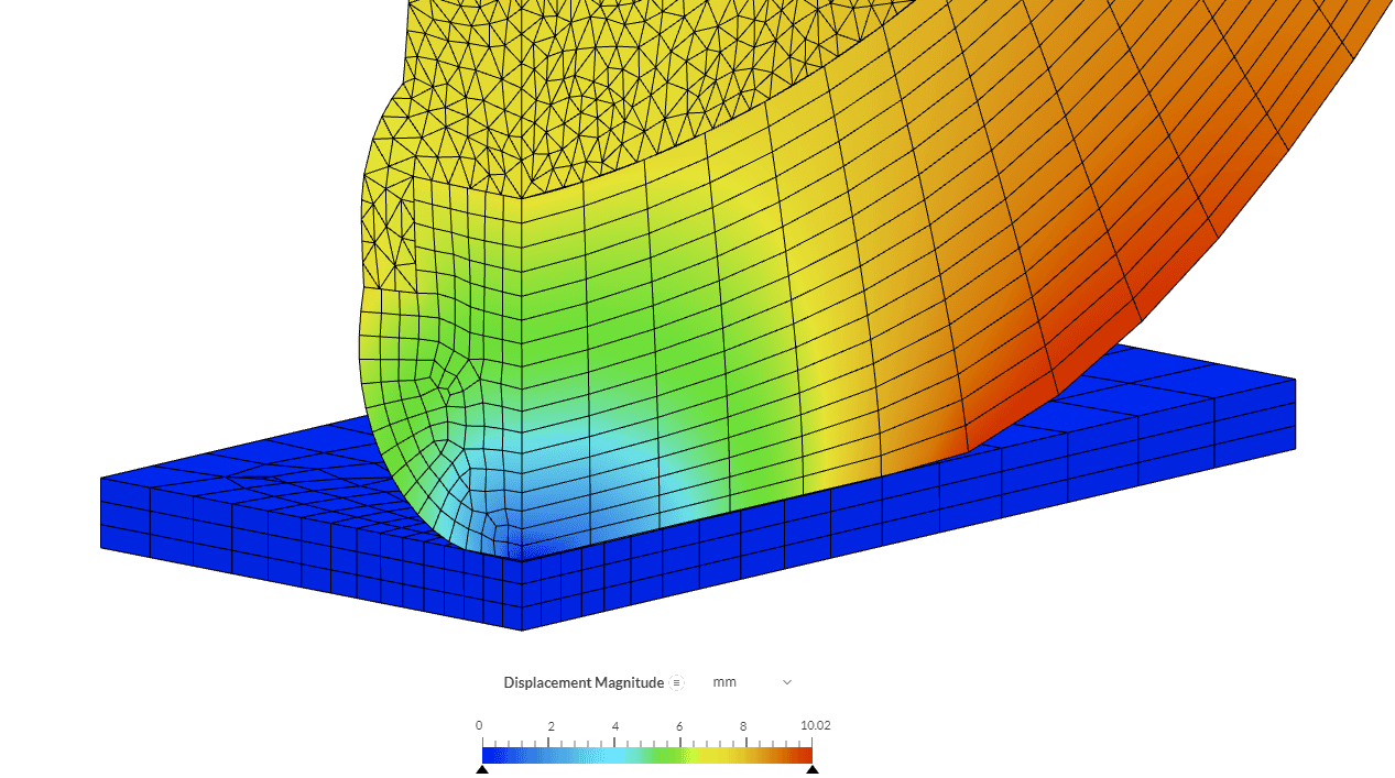
The details of the deformation of the tire in the region of contact with the ground are well appreciated.

6.3 Animation of the Results

We can visualize the loading and unloading process and the evolution of the deformation by creating an Animation filter, the same way we added the Displacement filter (see Figure 34):

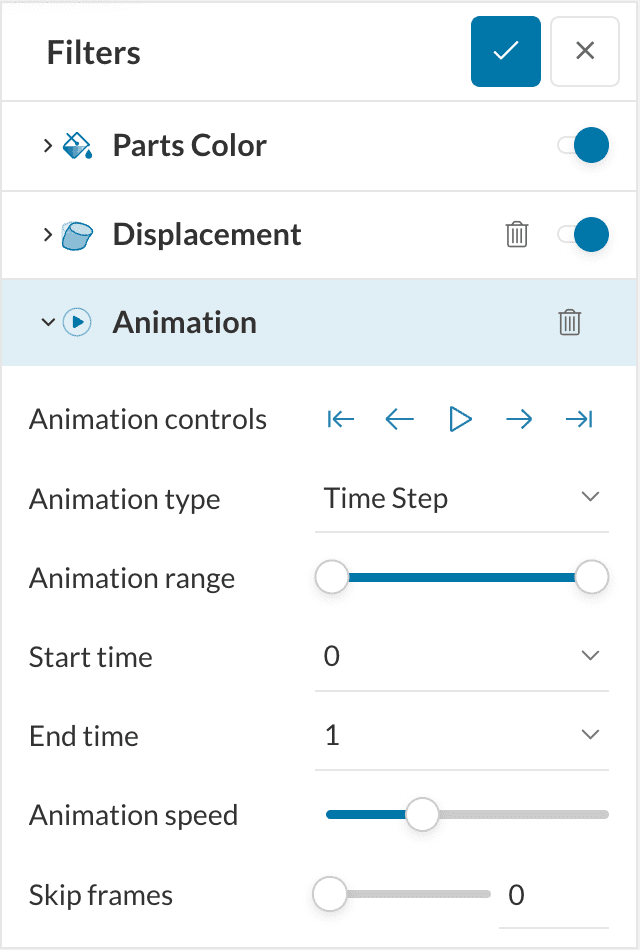
The default parameters are enough for our purpose. Click the ‘Play’ button to start the animation and you should see something as shown:

Animation 1 shows the deformation process and the corresponding contour plot for the von Mises stress. The effect of the load curve and the points of maximum deformation and stress can be appreciated.

Finally, we can take a look at the load vs. deformation plot, created locally by measuring the displacement of a point at the center of the wheel in post-processing tool Paraview, and using the known force curve:

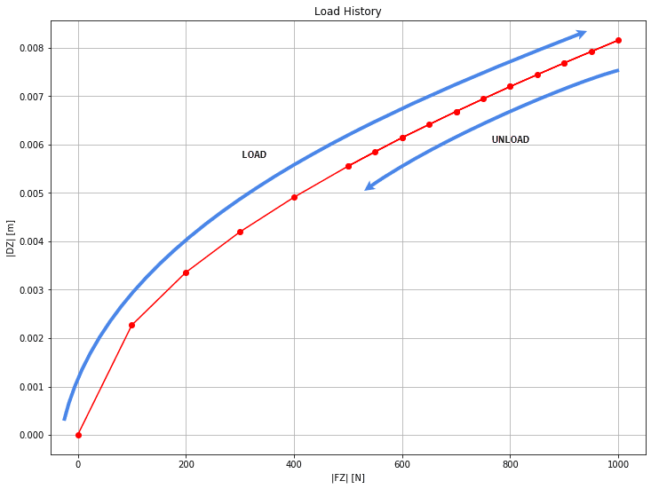
Figure 38 shows the vertical displacement magnitude of a point at the load application face, versus the applied load magnitude. Here, the nonlinear behavior of the model can be clearly seen, with the curvature of the load vs displacement curve following the hyperelastic behavior on the loading and unloading steps.

If you want to learn more about SimScale’s online post-processor, you can have a look at our dedicated guide:

Integrated Post-Processor

Congratulations, you finished the differential casing tutorial!

Last updated: July 23rd, 2025