How to Generate Particle Traces and Slices in PWC Analysis?

In PWC analysis, the main goal is to generate pedestrian wind comfort results. To be able to see the flow results for other regions within the domain, the user has to set “Additional results”. This article explains how to set a PWC analysis to be able to generate particle traces (streamlines) and slices.

Please visit the documentation page to learn more about the Pedestrian Wind Comfort Analysis type.

Solution

1. Region of Interest and Flow Domain

Region of interest (ROI) defines the area around the main building on which the pedestrian comfort should be evaluated.

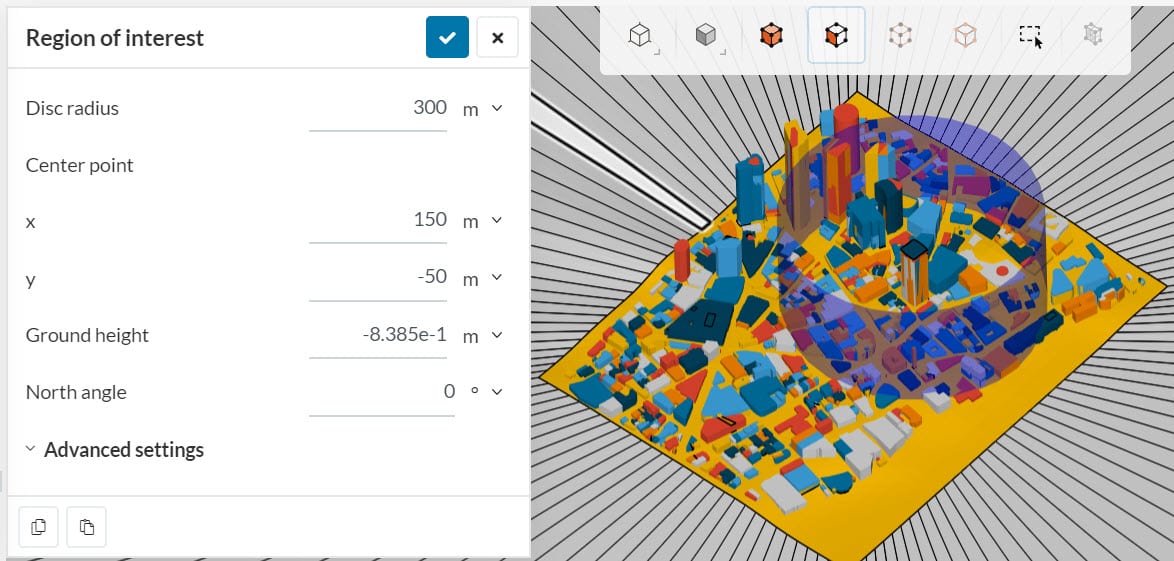
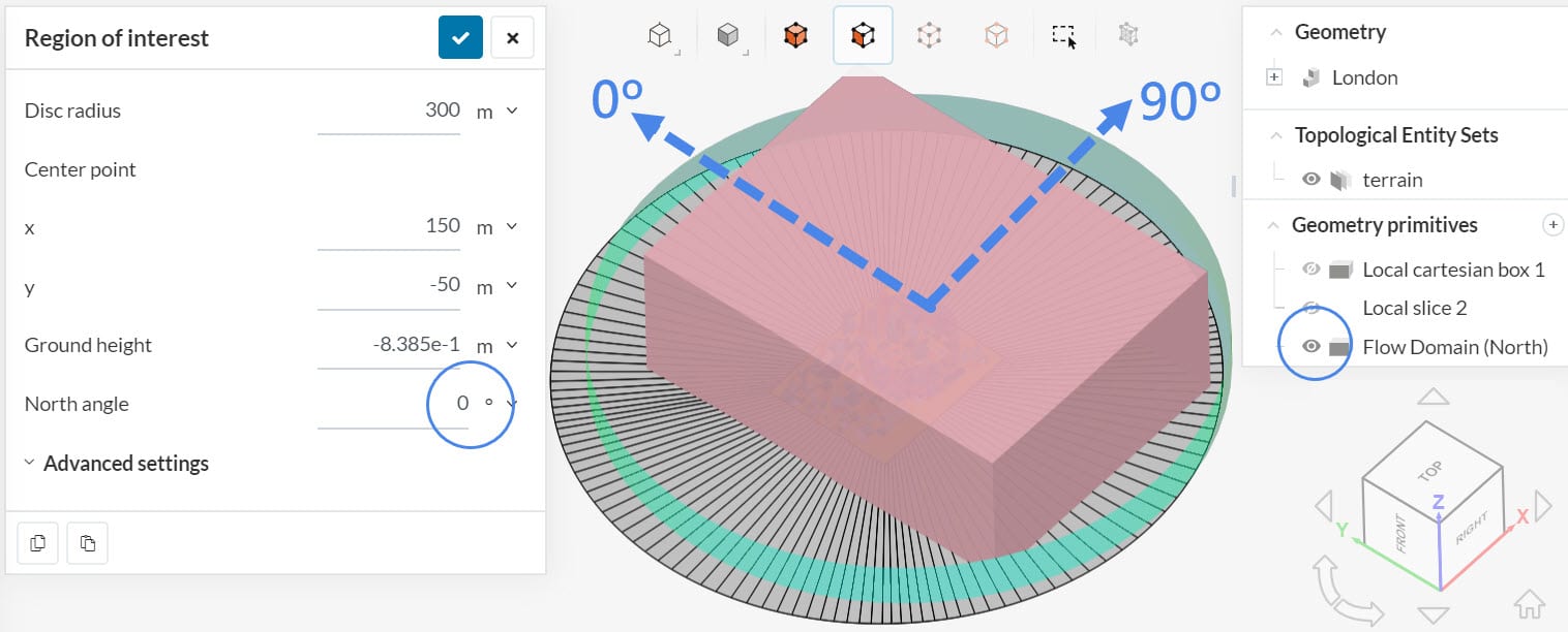
Once you define the ROI, you will be able to see the Flow domain (Wind tunnel) around it by clicking the eye icon.

In PWC analysis, the LBM solver by Pacefish®\(^1\) calculates the aerodynamics effects inside the flow domain and generates a comfort map. Even though the solver calculates the velocity, pressure, and turbulence values, it does not automatically saves all the data due to the storage space concerns. The user needs to define a region and set additional results for export.

2. Geometry Primitives

2.1 Local Cartesian Box

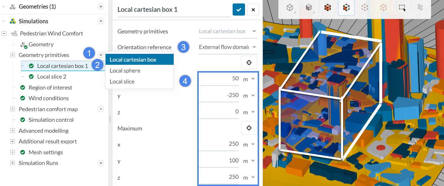
The aim of particle traces is to track the flow path in three dimensions. Therefore, we need a 3D domain to generate them.

Create a Local cartesian box where you would like to visualize the particle traces. Change the Orientation reference to the External flow domain. This will ensure the box aligns itself automatically, with respect to different wind directions.

Saving the additional data in 3D creates a larger results file. You may run out of disk space. Therefore, we strongly recommend keeping the box as small as possible to prevent an increase in simulation time and costs.

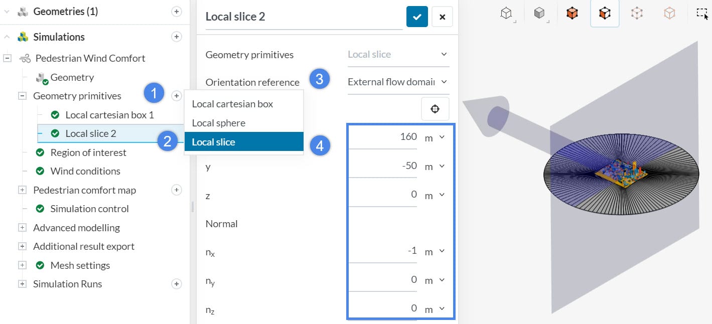
2.2 Local Slice

Particle traces is not the only way to observe the flow effects. Similarly, you can create 2D planes and visualize the data on them. Create a Local slice, where you would like to place the contours. Similarly, change the Orientation reference to the External flow domain.

3. Additional Result Export

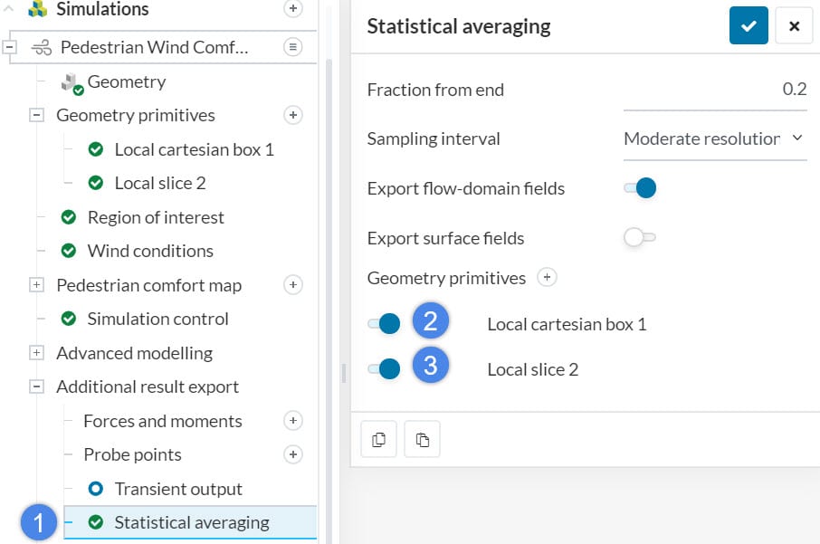
As we mentioned earlier, the solver does not save the flow parameters inside the whole domain. You need to save them additionally. You can either save transient results (Transient output) or steady-state results (Statistical averaging). Statistical averaging uses the results from last time steps, takes the average, and saves them for one time. Due to the storage, computation time, and cost concerns, we strongly recommend saving the results only in statistical averaging.

Activate the local cartesian box and/or the local slice you created before. Saving these results will allow you to create particle traces and slices in PWC analysis.

To learn more about the result control, please visit the following documentation page: Incompressible LBM (Lattice Boltzmann Method) Advanced Options

3.1 Fraction From End

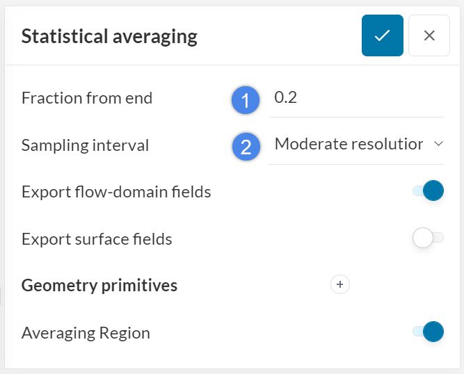
Pedestrian Wind Comfort (PWC) or Incompressible (LBM) analysis are developed to capture the transient behavior of a flow. Under the Transient output and Statistical averaging are Additional result exports. If you click one of these two, you will see the following settings:

• Fraction from end: Taking the simulation end time as a reference, how large the time frame should be?
• Sampling interval: How often should the data be saved.

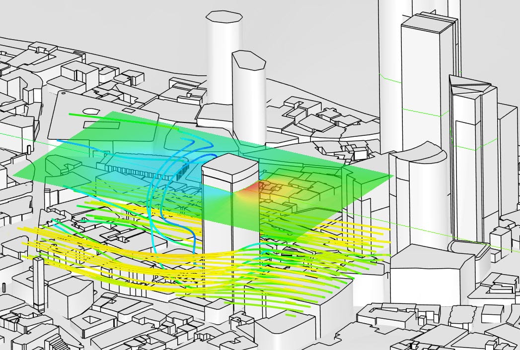
In a transient flow analysis (time-dependent), initial time steps are unsteady. During the early fluid passes, we expect to see the flow development. In other words, the flow field is still not steady. In the final fluid pass, we assume that the flow will reach a steady-state (time-independent). The time-independent result is what we need to achieve. Fraction from end defines the last fraction of the total simulation time. As an example, assigning 0.2 ensures that only the last 20% fraction of the results will be saved. The picture below shows the side view of a flow over the buildings with respect to different times.

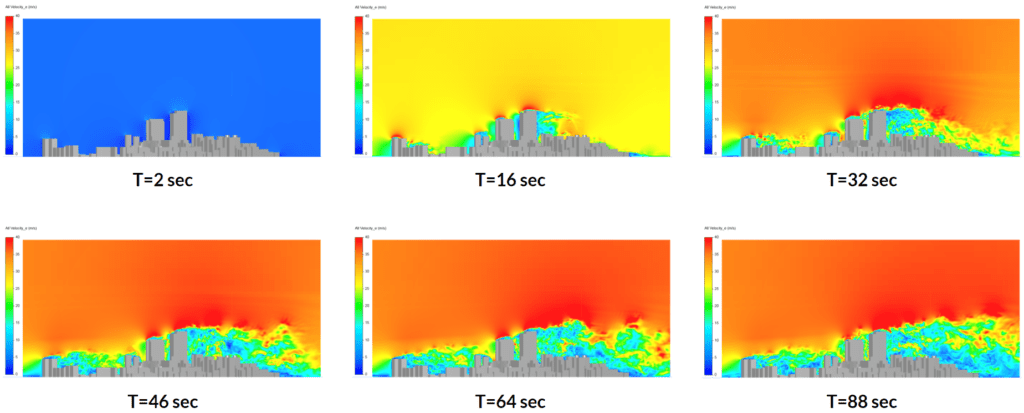
Figure 8 clearly shows the transient behavior of the flow. During the initial phase (up to 32 seconds), the flow is being developed. Later on, we do not see much change in the flow field, which means that the flow field reached a steady-state. Keep in mind that this is only a vertical slice, therefore we do not see the status of the rest of the domain. Usually, using at least 3 fluid passes and saving the last 20% fraction of the simulation results is convenient to extract useful results.

4. Results

You can see the results once the simulation is finished. Additional results are always saved per wind direction. Therefore, you need to choose a wind direction and navigate to Additional results.

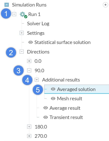
4.1 Generate Particle Traces

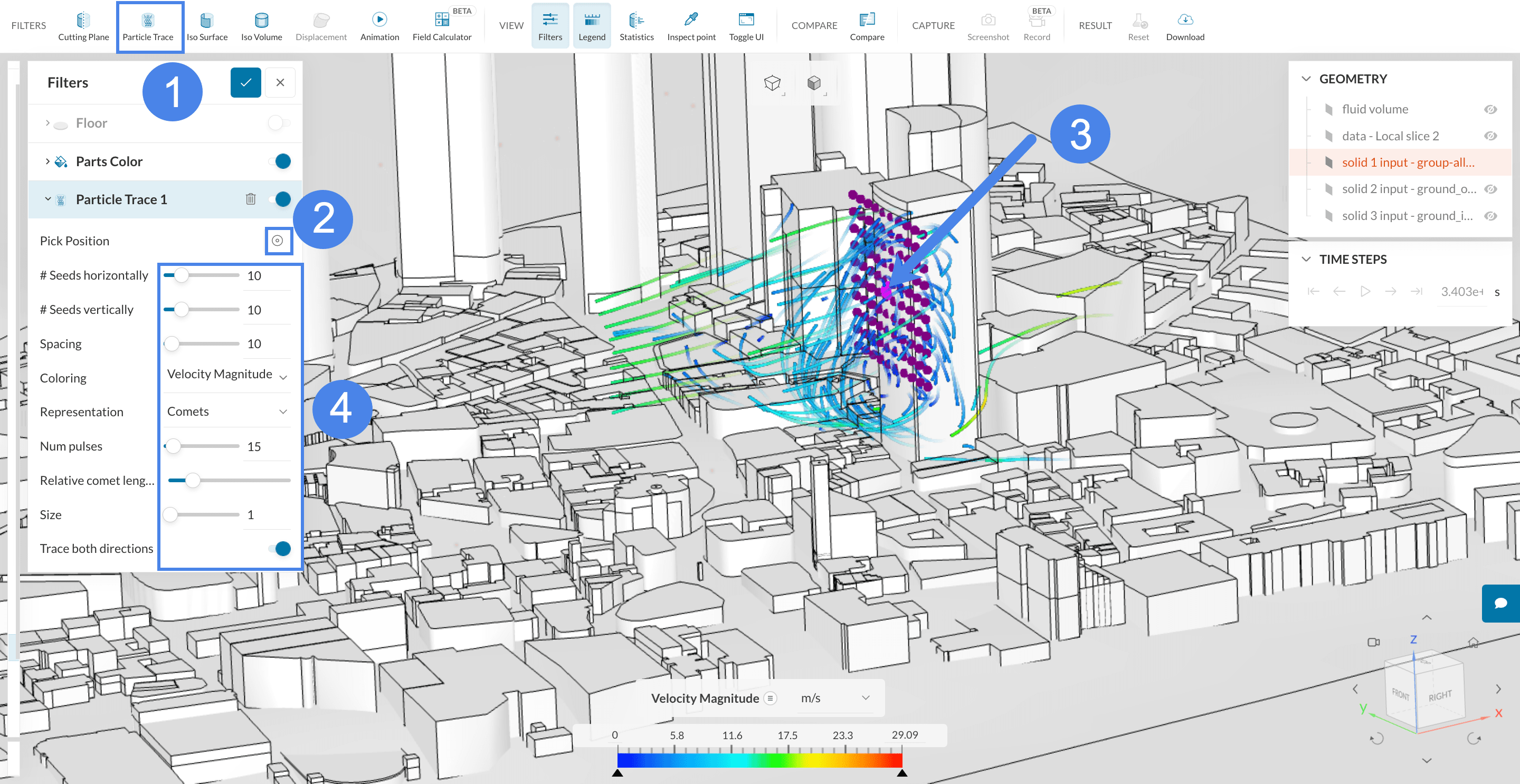
Once you are in Solution fields, you will see a green box. This is the Local cartesian box you defined under Geometry primitives. Velocity and pressure values are saved in this region.

1. Select the ‘Particle Trace’ filter on the top of the page to get started.
2. Click the ‘Pick’ button.
3. Place the seeds on a flat surface. This surface should be on or inside the flow domain.
4. Adjust the number of seeds, size, type, and space in between them.

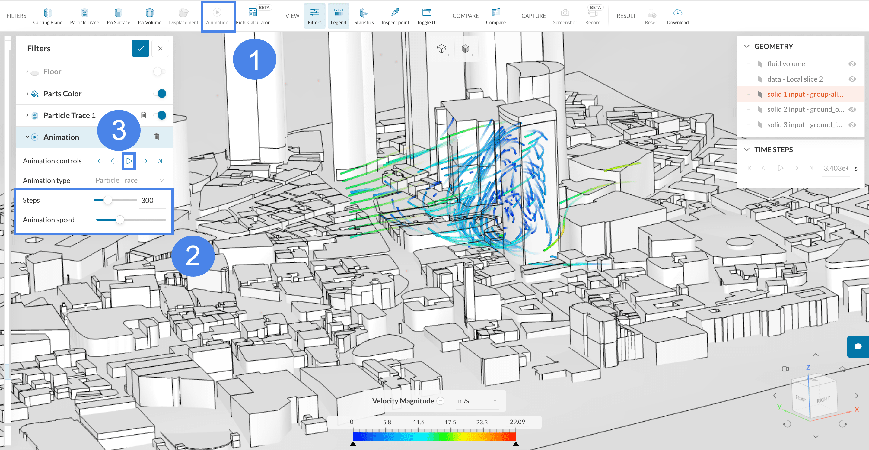
After capturing a nice view, you can animate the particle traces. First, create an ‘Animation’, then define the number of steps and animation speed, and finally, click the play button.

4.2 Generate Contours on a Slice

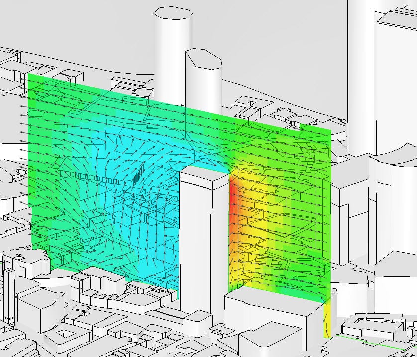
If you set a slice under the Additional Results before you created your run, then you can use it to visualize the flow parameters on it. Initially, ensure that your Local slice is visible.

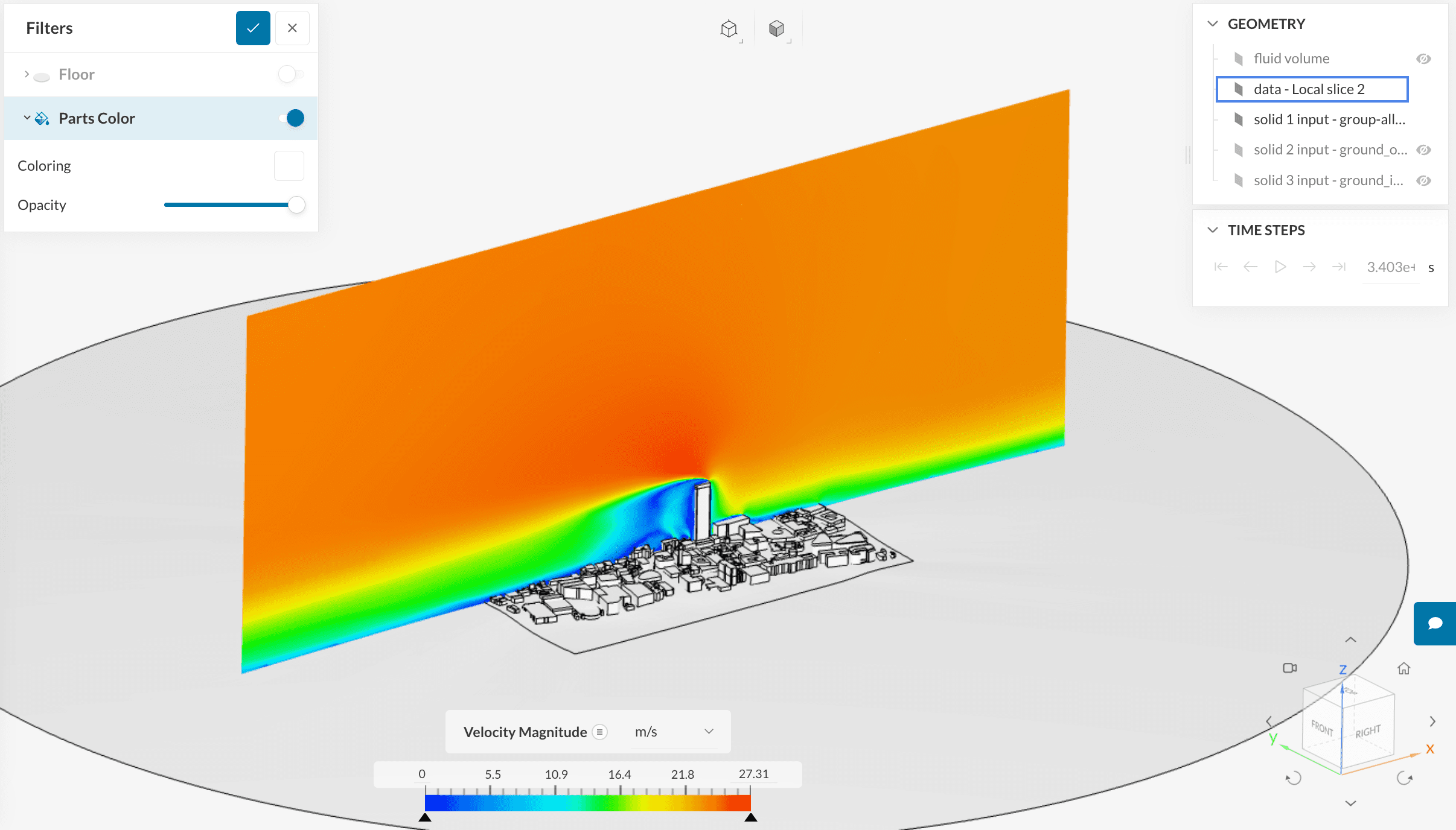
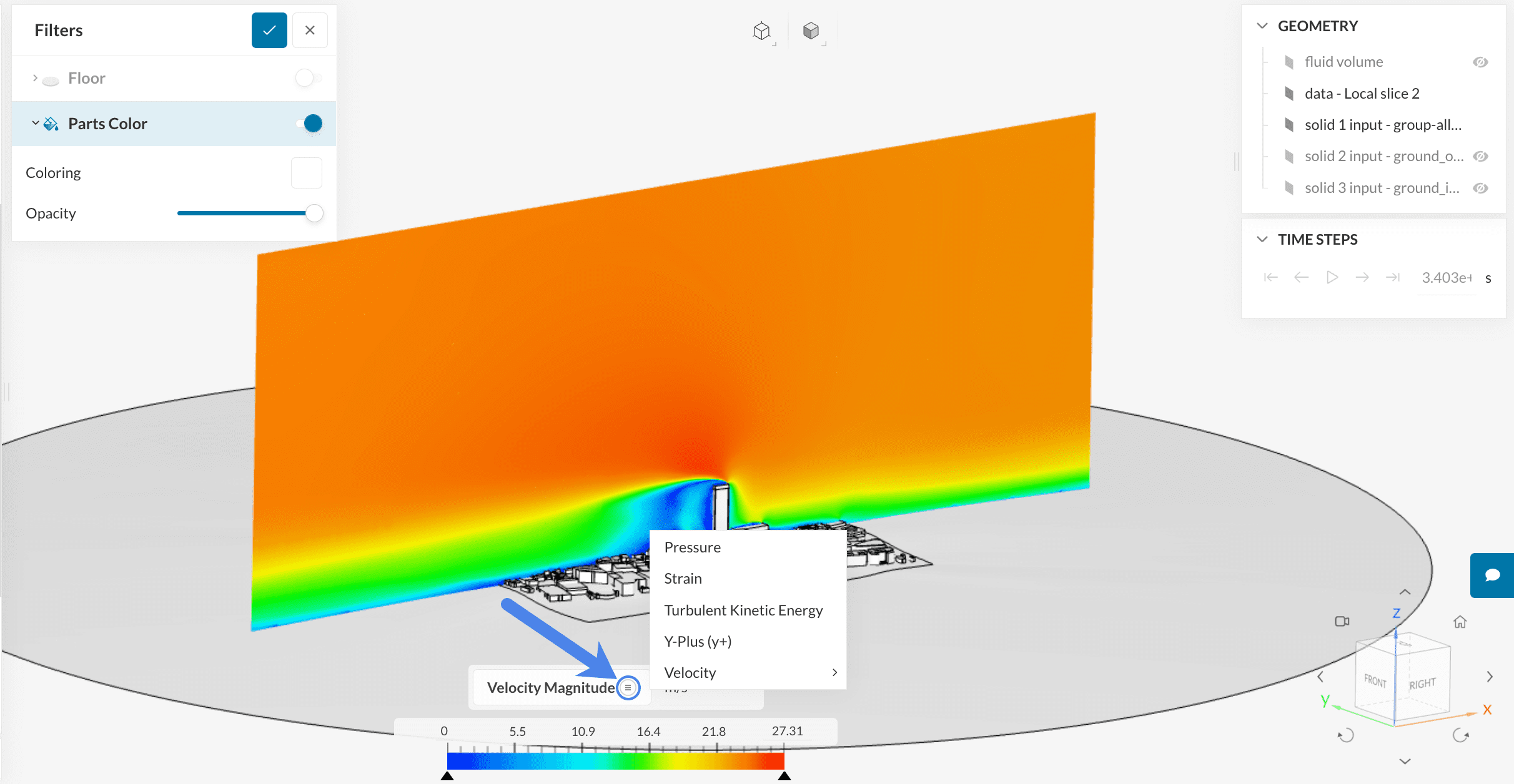
Apart from the velocity, you can select other parameters to be visualized, from this menu:

Best Practices

• Firstly, make sure the Orientation Reference for the geometry primitives selected is selected as the External flow domain.
• Secondly, avoid large boxes due to the storage and simulation costs concerns.
• Finally, statistical averaging is useful enough for additional results. Above all, the transient output might cause storage issues or an increase in simulation costs.