What Is FEA | Finite Element Analysis?
The Finite Element Analysis (FEA) is the simulation of any given physical phenomenon using the numerical technique called the Finite Element Method (FEM). Engineers use FEA software to reduce the number of physical prototypes and experiments and optimize components in their design phase to develop better products faster while saving on expenses.
With SimScale’s cloud-native platform, engineers can perform structural analysis using FEA directly in their web browser, enabling fast, scalable, and collaborative simulations without the need for expensive hardware or software installations.
It is necessary to use mathematics to comprehensively understand and quantify any physical phenomena such as structural or fluid behavior, thermal transport, wave propagation, the growth of biological cells, etc. Most of these processes are described using Partial Differential Equations (PDEs). However, for a computer to solve these PDEs, numerical techniques have been developed over the last few decades, and one of the prominent ones today is the Finite Element Analysis.
Differential equations not only describe natural phenomena but also physical phenomena encountered in engineering mechanics. These partial differential equations (PDEs) are complicated equations that need to be solved in order to compute relevant quantities of a structure (like stresses (\(\epsilon\)), strains (\(\epsilon\)), etc.) in order to estimate the structural behavior under a given load. It is important to know that FEA only gives an approximate solution to the problem and is a numerical approach to getting the real result of these partial differential equations.
Simply, FEA is a numerical method used for the prediction of how a part or assembly behaves under given conditions.
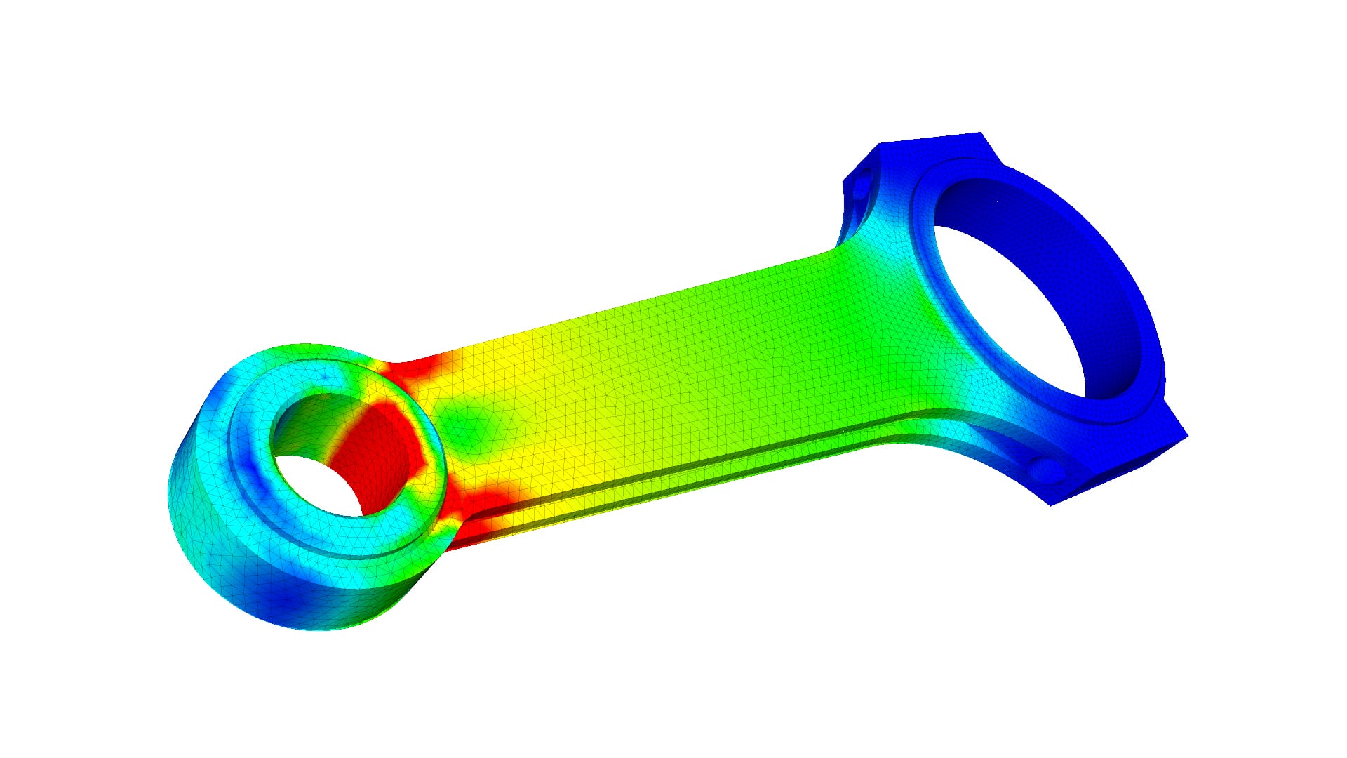
It is used as the basis for modern simulation software and helps engineers find weak spots, areas of tension, etc., in their designs. The results of a simulation based on the FEA method are usually depicted via a color scale that shows, for example, the pressure distribution over the object.
Depending on one’s perspective, FEA can be said to have its origin in the work of Euler as early as the 16th century. However, the earliest mathematical papers on Finite Element Analysis can be found in the works of Schellbach [1851] and Courant [1943].
FEA was independently developed by engineers in different industries to address structural mechanics problems related to aerospace and civil engineering. The development of FEA for real-life applications started around the mid-1950s, as papers by Turner, Clough, Martin & Topp [1956], Argyris [1957], and Babuska & Aziz [1972] show. The books by Zienkiewicz [1971] and Strang & Fix [1973] also laid the foundations for future developments in FEA software.
Divide and Conquer: Approximations for FEA
To be able to make simulations, a mesh consisting of up to millions of small elements that together form the shape of the structure needs to be created. Calculations are made for every single element. Combining the individual results gives us the final result of the structure.
The approximations we just mentioned are usually polynomials and, in fact, interpolations over the element(s). This means we know values at certain points within the element but not at every point. These ‘certain points’ are called nodal points and are often located at the boundary of the element. The accuracy with which the variable changes is expressed by some approximation, for example, linear, quadratic, and cubic.
In order to get a better understanding of approximation techniques, we will look at a one-dimensional bar. Consider the true temperature distribution T(x) along the bar in the picture below:
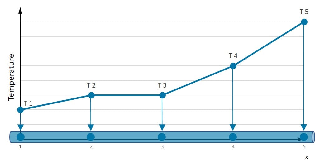
Let’s assume we know the temperature of this bar at five specific positions (Numbers 1-5 in the illustration). How can we predict the temperature between these points? A linear approximation is quite good, but there are better possibilities to represent the real temperature distribution.
If we choose a square approximation, the temperature distribution along the bar is much smoother. Nevertheless, we see that irrespective of the polynomial degree, the distribution over the rod is known once we know the values at the nodal points.
If we had an infinite bar, we would have an infinite amount of unknowns (DEGREES OF FREEDOM (DOF)). But in this case, we have a problem with a “finite” number of unknowns.
A system with a finite number of unknowns is called a discrete system.
A system with an infinite number of unknowns is called a continuous system.
For the purpose of approximations, we can find the following relation for a field quantity \(u(x)\):
$$ u(x) = u^h(x) + e(x) \tag{1}$$
Where \(u^h(x)\) is the approximation, which differs from the real solution \(u(x)\), and \(e(x)\) is the error term, which is not known before. De facto, this error term has to vanish so that the approximate solution \(u^h(x)\) becomes valid. The question that arises is how \(u^h(x)\) can be parametrized in a discrete function space. One possible solution is to express \(u^h(x)\) as a sum of shape function \(\phi_i(x)\) with coefficients \(\alpha_i(x)\).
$$ u^h(x) = \sum_{i=1}^n \alpha_i\phi_i(x) \tag{2}$$
The line illustrated at the top shows this principle for a 1D problem. \(u\) can represent the temperature along the length of a rod that is heated in a non-uniform manner. In our case, there are four elements along the x-axis, where the function defines the linear approximation of the temperature illustrated by dots along the line.
One of the biggest advantages of using the Finite Element Analysis is that we can either vary the discretization per element or discretize the corresponding basis functions. De facto, we could use smaller elements in regions where high gradients of \(u\) are expected. For the purpose of modeling the steepness of the function, we need to make approximations.
Partial Differential Equations (PDE)
Before proceeding with the FEA itself, it is important to understand the different types of PDEs and their suitability for FEA. Understanding this is important to everyone, irrespective of one’s motivation to use finite element analysis. One should constantly remind oneself that FEA software is a tool, and any tool is only as good as its user.
PDEs can be categorized as:
- Elliptic: they are quite smooth
- Hyperbolic: they support solutions with discontinuities
- Parabolic: they describe time-dependent diffusion problems
When solving these differential equations, boundary conditions and/or initial conditions need to be provided. Based on the type of PDE, the necessary inputs can be evaluated. Examples of PDEs in each category include the Poisson equation (Elliptic), Wave equation (Hyperbolic) and Fourier law (Parabolic).
There are two main approaches to solving elliptic PDEs – Finite Difference Analysis (FDA) and Variational (or Energy) Methods. FEA falls into the second category of variational methods. Variational approaches are primarily based on the philosophy of energy minimization.
Hyperbolic PDEs are commonly associated with jumps in solutions. The wave equation, for instance, is a hyperbolic PDE. Owing to the existence of discontinuities (or jumps) in solutions, the original FEA technology (or Bubnov-Galerkin Method) was believed to be unsuitable for solving hyperbolic PDEs. However, over the years, modifications have been developed to extend the applicability of FEA software and technology.
It is important to consider the consequence of using a numerical framework that is unsuitable for the type of PDE that is chosen. Such usage leads to solutions that are known as “improperly posed”. This could mean that small changes in the domain parameters lead to large oscillations in the solutions, or the solutions exist only on a certain part of the domain or time. These are not reliable.
Well-posed solutions are defined with a unique one that exists continuously for the defined data. Hence, considering reliability, it is extremely important to obtain them.
The Weak and Strong Formulation
The mathematical models of heat conduction and elastostatics covered in this series consist of partial differential equations with initial and boundary conditions. This is also referred to as the so-called Strong Form of the problem. A few examples of “strong forms” are given in the table below.
| Differential Equations | Physical problem | Quantities |
| \(\frac{d}{dx}\left(Ak\frac{dT}{dx}\right)+Q=0\) | One-dimensional heat flow | \(T\) = temperature, \(A\) = Area, \(k\) = thermal conductivity, \(q\) = heat supply |
| \(\frac{d}{dx}\left(AE\frac{du}{dx}\right)+b=0\) | Axially loaded elastic bar | \(u\) = displacement, \(A\) = Area, \(E\) = Young’s modulus, \(b\) = axial loading |
| \(S\frac{d{^2}w}{dx{^2}}+p=0\) | Transversely loaded flexible string | \(w\) = deflection, \(S\) = String force, \(p\) = lateral loading |
| \(\frac{d}{dx}\left(AD\frac{dc}{dx}\right)+Q=0\) | One-dimensional diffusion | \(c\) = ion contraction, \(A\) = area, \(D\) = diffusion coefficient, \(Q\) = ion supply |
| \(\frac{d}{dx}\left(A\gamma\frac{dV}{dx}\right)+Q=0\) | One-dimensional electric current | \(V\) = voltage, \(A\) = area, \(\gamma\) = electric conductivity, \(Q\) = electric charge supply |
| \(\frac{d}{dx}\left(A\frac{D{^2}}{32\mu}\frac{dp}{dx}\right)+Q=0\) | Laminar flow in pipe (Poiseuille flow) | \(p\) = pressure, \(A\) = area, \(D\) = diameter, \(mu\) = viscosity, \(Q\) = fluid supply |
Second-order partial differential equations demand a high degree of smoothness for the solution \(u(x)\). That means that the second derivative of the displacement has to exist and has to be continuous! This also implies requirements for parameters that can not be influenced, like the geometry (sharp edges) and the material parameters (different modulus in a material).
To develop the finite element formulation, the partial differential equations must be restated in an integral form called the weak form. The weak form and strong form are equivalent. In stress analysis, the weak form is called the principle of virtual work.
$$ \int^l_0\frac{dw}{dx}AE\frac{du}{dx}dx=(wA\overline{t})_{x=0} + \int^l _0wbdx ~~~ \forall w~with ~w(l)=0 \tag{3}$$
The given equation is the so-called weak form (in this case, the weak formulation for elastostatics). The name states that solutions to the weak form do not need to be as smooth as solutions of the strong form, which implies weaker continuity requirements.
You have to keep in mind that the solution satisfying the weak form is also the solution of the strong counterpart of the equation. Also, remember that the trial solutions \(u(x)\) must satisfy the displacement boundary conditions. This is an essential property of the trial solutions, and this is why we call those boundary conditions essential boundary conditions.
Do these formulations interest you? If yes, please read more in the forum topic about the equivalence between the weak and strong formulation of PDEs for FEA.
Minimum Potential Energy: The Variation Principle
The Finite Element Analysis can also be executed with the Variation Principle. In the case of one-dimensional elastostatics, the minimum potential energy is resilient for conservative systems. The equilibrium position is stable if the potential energy of the system \(\Pi\) is minimum. Every infinitesimal disturbance of the stable position leads to an energetic, unfavorable state and implies a restoring reaction.
An easy example is a normal glass bottle that is standing on the ground, where it has minimum potential energy. If it falls over, nothing is going to happen except for a loud noise. If it is standing on the corner of a table and falls over to the ground, it is rather likely to break since it carries more energy towards the ground. For the variation principle, we make use of this fact. The lower the energy level, the less likely it is to get the wrong solution. The total potential energy \(\Pi\) of a system consists of the work of the inner forces (strain energy)
$$ A_i = \int_0^l \underbrace{\frac{1}{2} E(x)A(x) \left(\frac{du}{dx} \right)^2}_{\frac{1}{2}\sigma\epsilon A(x)} dx \tag{4}$$
and the work of the external forces
$$ A_a = A(x)\overline{t}(x)u(x)|_{\Gamma _t} \tag{5}$$
The total energy is:
$$ \Pi = A_i – A_a \tag{6}$$
Find more about the minimum potential energy in our related forum topic.
Mesh Convergence
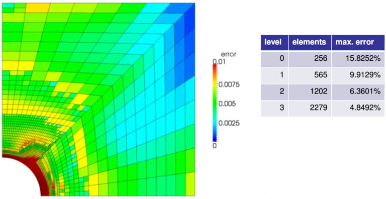
One of the most overlooked issues in computational mechanics that affect accuracy is mesh convergence. This is related to how small the elements need to be to ensure that the results of an analysis are not affected by changing the size of the mesh.
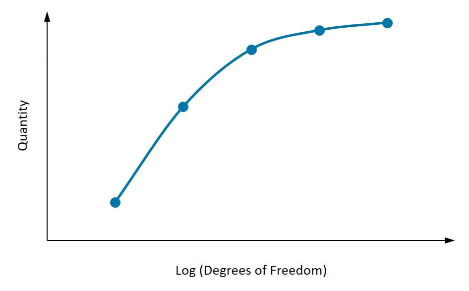
The figure above shows the convergence of a quantity with an increase in the degrees of freedom. As depicted in the figure, it is important to first identify the quantity of interest. At least three points need to be considered, and as the mesh density increases, the quantity of interest starts to converge to a particular value. If two subsequent mesh refinements do not change the result substantially, then one can assume the result to have converged.
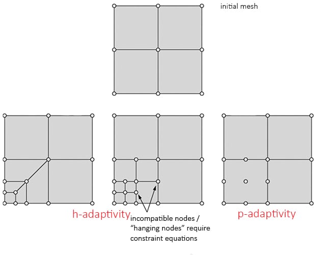
Going into the question of mesh refinement, it is not always necessary that the mesh in the entire model is refined. St. Venant’s Principle enforces that the local stresses in one region do not affect the stresses elsewhere. Hence, from a physical point of view, the model can be refined only in particular regions of interest and further have a transition zone from coarse to fine mesh.
There are two types of refinements (h-refinement and p-refinement), as shown in Figure 5 above. H-refinement relates to the reduction in the element sizes, while p-refinement relates to increasing the order of the element.
Here, it is important to distinguish between geometric effect and mesh convergence, especially when meshing a curved surface. Using straight (or linear) elements will require more elements (or mesh refinement) to capture the boundary exactly. Mesh refinement leads to a significant reduction in errors.
Refinement like this can allow an increase in the convergence of solutions without increasing the size of the overall problem being solved.
How to Measure Convergence?
So now that the importance of convergence has been discussed, how can convergence be measured? What is a quantitative measure of convergence? The first way would be to compare with analytical solutions or experimental results.
Error of the Displacements:
$$ e_u = u – u^h \tag{7}$$
where \(u\) is the analytical solution for the displacement field.
Error of the Strains:
$$ e_\epsilon = \epsilon – \epsilon^h \tag{8}$$
where \(\epsilon\) is the analytical solution for the strain field.
Error of the Stresses:
$$ e_\sigma = \sigma – \sigma^h \tag{9}$$
where \(\sigma\) is the analytical solution for the stress field.
As shown in the equations above, several errors can be defined for displacements, strains, and stresses. These errors could be used for comparison and would need to reduce with mesh refinement.
Learn more about mesh convergence in FEA and how errors are calculated with the respective norms for these quantities.
Finite Element Analysis Software
The Finite Element Analysis started with significant promise in modeling several mechanical applications related to aerospace and civil engineering. The applications of the Finite Element Method are just starting to reach their potential.
One of the most exciting prospects is its application to coupled problems like fluid-structure interaction: thermo-mechanical, thermo-chemical, thermo-chemo-mechanical problems, piezoelectric, ferroelectric, electromagnetics and other relevant areas.
Apply FEM yourself!
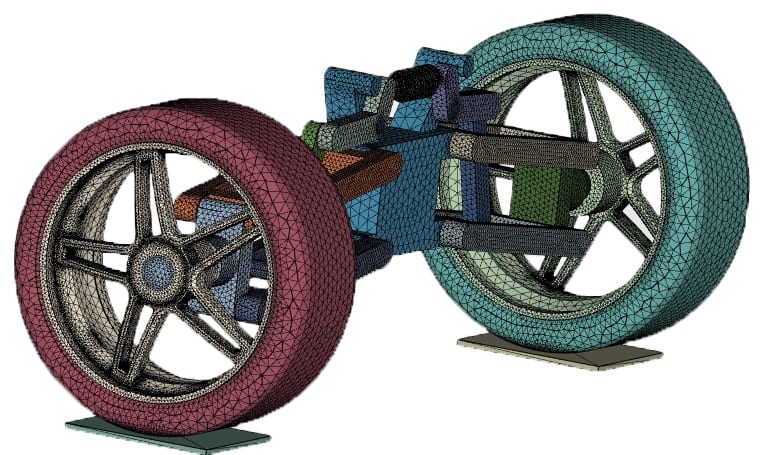
Do you also feel like applying finite element methods to real life scenarios, like a running wheel, or a drone, or a phone dropped accidentally. All of this is possible by simply signing up as our Community or Professional SimScale user.
Static Analysis
With static analysis, you can analyze linear static and nonlinear quasi-static structures. In a linear case with an applied static load, only a single step is needed to determine the structural response. Geometric, contact, and material nonlinearity can be taken into account. An example is a bearing pad of a bridge.
Dynamic Analysis
Dynamic analysis helps you analyze the dynamic response of a structure that experienced dynamic loads over a specific time frame. To model the structural problems in a realistic way, you can also analyze the impacts of loads as well as displacements. An example is the impact of a human skull, with or without a helmet.
Modal Analysis
Eigenfrequencies and eigenmodes of a structure due to vibration can be simulated using modal analysis. The peak response of a structure or system under a given load can be simulated with harmonic analysis. An example is a paving stone subjected to harmonic pressure.
Types of Finite Element Method (FEM)
As discussed earlier in the section on PDEs, traditional FEM technology has demonstrated shortcomings in modeling problems related to fluid mechanics, wave propagation, etc. Several improvements have been made over the last two decades to improve the solution process and extend the applicability of finite element analysis to a wide genre of problems. Some of the important ones still being used include:
Extended Finite Element Method (XFEM)
The Bubnov-Galerkin method requires continuity of displacements across elements. Problems like contact, fracture, and damage, however, involve discontinuities and jumps that cannot be directly handled by Finite Element Methods. To overcome this shortcoming, XFEM was born in the 1990s.
XFEM works through the expansion of the shape functions with Heaviside step functions. Extra degrees of freedom are assigned to the nodes around the point of discontinuity so that the jumps can be considered.
Generalized Finite Element Method (GFEM)
GFEM was introduced around the same time as XFEM in the ’90s. It combines the features of traditional FEM software and meshless methods. Shape functions are primarily defined in the global coordinates and further multiplied by partition-of-unity to create local elemental shape functions. One of the advantages of GFEM is the prevention of re-meshing around singularities.
Mixed Finite Element Method
In several problems, like contact or incompressibility, constraints are imposed using Lagrange multipliers. These extra degrees of freedom arising from Lagrange multipliers are solved independently. The equations are solved like a coupled system.
hp-Finite Element Method (hp-FEM)
hp-FEM is a combination of using automatic mesh refinement (h-refinement) and increase in the order of polynomial (p-refinement). This is not the same as doing h- and p- refinements separately. When automatic hp-refinement is used, and an element is divided into smaller elements (h-refinement), each element can have different polynomial orders as well.
Discontinuous Galerkin Finite Element Method (DG-FEM)
DG-FEM has shown significant promise for using the idea of Finite Elements for solving hyperbolic equations where traditional Finite Element Methods have been weak. In addition, it has also shown promise in bending and incompressible problems which are commonly observed in most material processes. Here, additional constraints are added to the weak form, including a penalty parameter (to prevent interpenetration) and terms for other equilibrium of stresses between the elements.
Interested in reading more FEA-related content?
FEA in SimScale
The FEA software component of SimScale enables you to virtually test and predict the behavior of structures and hence solve complex structural engineering problems subjected to static and dynamic loading conditions. This FEA simulation platform uses scalable numerical methods that can calculate mathematical expressions that would otherwise be very challenging due to complex loading, geometries, or material properties.
References
- Jacob Fish and Ted Belytschko, “A First Course in Finite Elements by Jacob Fish and Ted Belytschko”, Wiley, 2007
- R . Courant, “Variational methods for the solution of problems of equilibrium and vibrations”, 1943
- K . Schellbach, “Probleme der Variationsrechnung”, 1851, Berlin
Last updated: April 13th, 2026
Did this article solve your issue?
How can we do better?
We appreciate and value your feedback.
What's Next
What is von Mises Stress?

