After a long break I am back with a new interesting post about the Weak and Strong forms in the Finite Element Method!
Introduction
The mathematical models of heat conduction and elastostatics covered in Chapter 2 of this series consist of (partial) differential equations with initial conditions as well as boundary conditions. This is also referred to as the so called Strong Form of the problem. In this chapter we shall therefore discuss the formulation in terms of so-called strong and weak forms. To facilitate this, we consider simple differential equations, which turns out to govern one-dimensional heat flow as well as other physical phenomena like elastic bars, flexible stringt, etc. To obtain a firm background, it is convenient first to establish this differential equation. So let’s get started!!!
The partial differential equations in the last paragraph are second order partial differential equations. This demands a high degree of smoothness for the solution u(x). That means that the second derivative of the displacement has to exist and has to be continuous! This also implies requirements for parameters that are not influenceable like the geometry (sharp edges) and material parameters (different Young’s modulus in a material).
The idea now is to formulate the continuous problem as an integral!
The strong form for an axially loaded bar
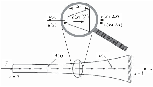
Consider the static response of an elastic bar with variable cross section as shown in the picture above. This is an example of a problem in linear stress analysis or linear elasticity, where we seek to find the stress distribution \sigma(x) in the bar. The stress will result from the deformation of the body, which is characterized by the displacement of points in the body, u(x). This displacement implies a strain denoted by \epsilon(x). You can see in the picture that the body is subjected to a body force or distributed loading b(x) (units are force per length). In addition, we can describe the body force which could be due to gravity. Furthermore, loads can be prescribed at the ends of the bar, where the displacement is not prescribed \rightarrow these loads are called tractions and denoted by \overline{t} (units are force per area \rightarrow multiplied with an area give us the applied force).
The bar must satisfy the following conditions:
- Equilibrium must be fulfilled
- Stress-Strain law must be satisfied. \sigma(x) = E(x)\epsilon(x)
- Displacement field must be compatible
- Strain-Displacement equations must be satisfied
The differential equation of this bar can be obtained from equilibrium of external forces b(x) as well as the internal forces p(x) acting on the body in the axial direction (along x-axis).
Summing the forces in x-direction:
Rearranging the terms:
The limit of this equation with \Delta x \rightarrow 0 makes the first term the derivative dp/dx and the second term becomes b(x). So we can write:
This equation expresses the equilibrium equation in terms of the internal force p. Stress is defined as:
The strain-displacement equation is obtained by:
Taking the limit of above for \Delta x \rightarrow 0, we see that:
The stress-strain law, also known as Hooke’s law has already been introduced in earlier chapters:
Substituting (3) in (4) and that result into (1) yields:
Equation (5) is a second-order ordinary differential equation. u(x) is the dependent variable, which is the unknown function, and x the independent variable. Equation (5) is a specific form of equation (1). Equation (1) applies both linear and nonlinear materials whereas (5) assumes linearity in the definition of the strain (3) and stress-strain law (4). Compatibility is satisfied by requiring the displacement to be continuous.
To solve the differential equation, we need to prescribe boundary conditions at the two ends of the bar. At x = l , the displacement, u(x=l), is prescribed; at x = 0 , the force per unit area, or traction, denoted by \overline t, is prescribed. We write these conditions as:
Note that the lines above the letters indicate a prescribed boundary value.
The traction \overline t has the same units as stress (force/area), but its sign is positive when it acts in the positive x-direction regardless of which face it is acting on, whereas the stress is positive in tension and negative in compression, so that on a negative face a positive stress corresponds to a negative traction.
The governing differential equation (5) along with the boundary conditions (6) is called the strong form of the problem.
To summarize, the strong form consists of the governing equation and the boundary conditions, which for example are
The weak form (1D)
To develop the finite element formulation, the partial differential equations must be restated in an integral form called the weak form. The weak form and the strong form are equivalent! In stress analysis the weak form is called the principle of virtual work.
We start by multiplying the governing equation (7a) and the traction boundary condition (7b) by an arbitrary function w(x) and integrating over the domains on which they hold: for the governing equation, the pertinent domain is [0,l]. For the traction boundary, it is the cross-sectional area at x = 0 (no integral needed since this condition only holds only at a point but we multiply it with A). The results are:
The function w is called weight function or test function. In the above, \forall w denotes that w(x) is an arbitrary function, i.e. (13) has to hold for all functions w(x). Arbitrariness of the weight function is crucial for the weak form. Otherwise the strong form is NOT equivalent to the weak form.
We did not enforce the boundary condition on the displacement in (13) by the weight function. It will be seen that it is easy to construct trial solutions u(x) that satisfy this boundary condition. We will also see that all weight functions satisfy
In solving the weak form, a set of admissible solutions u(x) that satisfy certain conditions is considered (also called trial solutions or candidate solutions). We could use equation (13) to construct a FEM method. But since we have the second derivative of $u(x)$$ in the equation, we would need very smooth trial functions which are difficult to construct in more than one dimension.
The resulting stiffness matrix would also be not symmetric! We will transform (13) into a form containing only first derivatives. This will give us a symmetric stiffness matrix and allows us to use less smooth solutions.
We rewrite (13a) in an equivalent form:
Applying integration by parts on equation (15):
Using (16),equation (15) can be written as:
We note that by the stress-strain law and strain-displacement equations, the underscored boundary term is the stress \sigma:

The first term in equation (18) vanishes since we assumed w(l)=0: for that reason is it useful to construct weight functions that vanish on prescribed displacement boundaries. Though the term looks insignificant, it would lead to loss of symmetry in the final equation. Form (13b), we can see that the second term equals (wA\overline t)_{x=0}, so equation (18) becomes
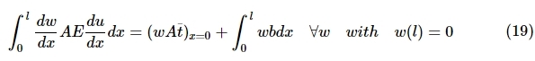
To summarize the approach: We multiplied the governing equation and traction boundary by an arbitrary, smooth weight function and integrated the products over the domain where they hold. We also transformed the integral so that the derivatives are of lower order.
The crux of this approach: Trial solutions that satisfy the equation developed for all smooth w(x) with w(l)=0 is the solution. We obtain the solution as follows:
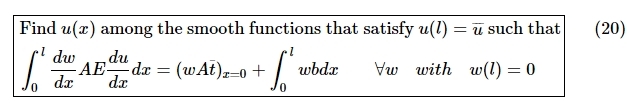
Equation (20) is called the weak form. The name states that solutions to the weak form do not need to be as smooth as solutions of the strong form. \rightarrow weaker continuity requirements
You have to keep in mind that the solution satisfying equation (20) is also the solution of the strong counterpart of this equation. Also remember that the trial solutions u(x) must satisfy the displacement boudary conditions. This is an essential property of the trial solutions and that is why we call those boundary conditions essential boundary conditions. The traction boundary conditions emanate naturally from equation (20) which means that the trial solutions do not need to be constructed to satisfy the traction boundary condition. These boundary conditions are therefore called natural boundary conditions.
A trial solution that is smooth AND satisfies the essential boundary conditions is called admissible. A weight function that is smooth AND vanishes on essential boundaries is admissible. When weak forms are used to solve a problem, the trial solutions and weight functions must be admissible. Also notice that equation (20) is symmetric in w and u which will lead to a symmetric stiffness matrix. The highest order derivative that appears in this equation is of first order!
Continuity
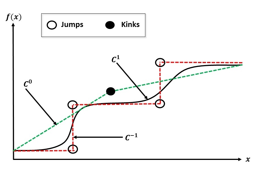
In this chapter I will shortly explain the differences and concepts of smothness, i.e. continuity. A function is called a C^n function if its derivatives of order j for 0\leq j \leq n exist and are continous functions in the entire domain. We will be concerned mainly with C^0, C^{-1} and C^1 functions. Examples are illustrated in the picture below. You can see that a C^0 function is piecewise continuously differentiable, i.e. its first derivative is continuous except at selected points. The derivative of a C^0 function is a C^{-1} function.
Examples:
-
If the displacement is a C^0 function, the strain is a C^{-1} function.
-
If the temperature field is a C^0 function, the flux is a C^{-1} function if the conductivity is C^0.
The derivative of a C^n is a C^{n-1} function.
As the superscript increases the progression of smoothness increases as well. So a C^{-1} function can have kinks and jumps. A C^0 function has no jumps but has kinks. A C^1 function has no kinks or jumps. In literature, jumps are often called strong discontinuities, whereas kinks are called weak discontinuities.
CAD Databases: CAD databases usually employ functions that are at least C^1; the most common are spline functions. Otherwise, the surface would possess kinks stemming from the function description, e.g. in a car there would be kinks in the sheet metal wherever C^1 continuity is not observed. Finite Elements usually employ C^0 functions.
The equivalence between the weak and strong forms
In the previous section, we constructed the weak and strong form. Now we will show the equivalence of both forms by showing that the weak form implies the strong form. This will insure that when we solve the weak form, then we have a solution to the strong form.
We can simply prove that the weak form implies the strong form by reversing the steps we used to obtain the weak form. So instead of using the integration by parts to eliminate the 2nd derivative of u(x), we reverse the formula to obtain an integral with a higher derivative and a boundary term. For this purpose, interchange the terms given in equation (17):
Substituting above in equation (20) and placing the integral terms on the left-hand side and the boundary terms on the right-hand side gives:
The quintessence making the proof possible is the arbitrariness of w(x). First we let
where \psi(x) is smooth, \psi(x) > 0 on 0 < x < l and \psi(x) vanishes on the boundaries. An example of a function satisfying the above requirements is \psi(x) = x(l-x). Because of how \psi(x) is constructed, it follows that w(l) = 0, so that w=0 on the prescribed displacement boundary, the essential boundary, is met.
Inserting (22) in (21) yields:
The boundary term vanishes because we have constructed the weight function so that w(0)=0. As the integrand in (23) is the product of a positive function and the square of a function, it must be positive at every point in the problem domain. The only way equality is met in equation (23) is if the integrand is zero at every point! It follows that:
which is exactly the strong form we had in the beginning \rightarrow Equation (5)
From (24) it follows that the integral in (21) vanishes, so we are left with
As the weight function is arbitrary, we select it such that w(0) = 1 and w(l)=0. It is very easy to construct such a function. (l-x)/x is a suitable weight function. Any other smooth function that you can draw in the interval [0,l] that vanishes at x=l is also suitable!
Since the cross-sectional area A(0)\neq 0 and w(0) \neq 0, it follows that
which is the natural boundary condition. \rightarrow Equation (7b)
The last remaining equation of the strong form, the displacement boundary condition (3.7c), is satisfied by all trial solutions by construction, which can be seen from (20) as we required u(l)=\overline u. Therefore, we can conclude that the trial solution that satisfies the weak form also sastisfies the strong form.
There are also other ways to prove the equivalence which are not covered in this “short” course but can be found in the book by Fish & Belytschko or in the book by Ottosen & Petersson.
Minimum Potential Energy
We can also motivate the FEM with a variational principle. In the case of one dimensional elastostatics the minimum of potential engery holds for conservative systems. The equilibrium position is stable if the potential energy of the system \Pi is a minimum. Every infinitesimal disturbance of the stable position leads to an energetic unfavourable state and implies a restoring reaction. The total potential energy \Pi of a system consists of the work of the inner forces (strain energy)
and the work of the external forces
The total energy is:
The condition for a minimum of the total potential energy is:
where u is an arbitrary solution which is compatible with the boundary conditions. u^* is the displacement field for which a minimum will be generated.
When disturbing the solution we get:
where \lambda \in \mathbb{R} is the amplitude of the disturbance and w(x) the test function with w=0 on the Dirichlet boundary. The test functions w(x) have to be from the Sobolev space \mathcal{H}_0^1.
Since \Pi is minimal for u^* we have:
This also has to hold for infinitesimal disturbances \lambda \rightarrow 0, \lambda \neq 0. The necessary condition for a minimum is then:
The expression above is also known as a Gâteaux derivative.
which gives us with the binomial formula:
Formula (27) with \lambda \rightarrow 0 gives us:
which gives us after some easy calculations
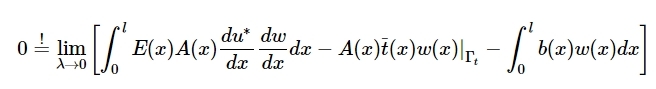
Since \lambda \rightarrow 0 and \lambda \neq 0 apply at the same time we have an equivalence to the strong form. So if a function u^*(x) is solving the minimization problem it automatically fulfils the weak form and vice versa.
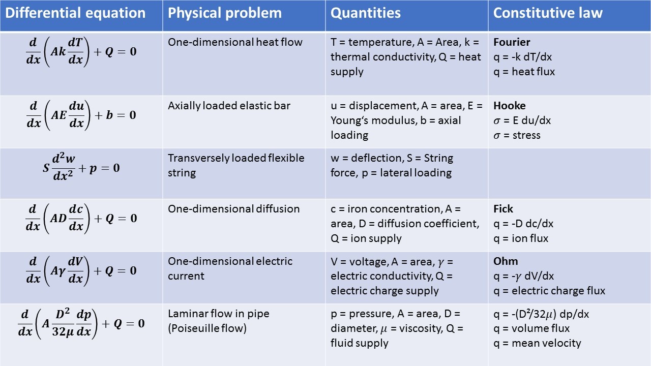
Examples of 2nd order differential equations
Concluding remarks
We can show for various physical problems that the methods we used are applicable since they all lead to the same type of differential equation and boundary condition and together are referred to as the strong form of the problem. We also showed that this so called strong form could be reformulated into an equivalent weak form.
I emphasized that the weak form is the one on which the FE approach is based. The reason is that the order of differentiation of the unknown is lower in the weak form than in the strong form, thus facilitating the approximation process.
The weak form applies without changes to continuous as well as discontinuous problems, implying the important conclusion that the FE method also holds for continuous as well as discontinuous problems.
Sources:
• Introduction to the Finite Element Method - Niels Ottosen & Hans Petersson
• A First Course in Finite Elements by Jacob Fish and Ted Belytschko
• Lectures of KIT Karlsruhe (Script: Einführung in die Finite Elemente Methode Sommersemester 2014)
This was the fifth part for FEM fundamentals.
If you find any mistakes or have wishes for the next chapters please let me know.
If you like a homework for this chapter just comment and I will set up some small problems that you can solve and we discuss it in this thread!
Scientia potentia est!
First chapter: The Finite Element Method - Fundamentals - Introduction [1]
Second chapter: The Finite Element Method - Fundamentals - Physical Problems [2]
Third chapter: The Finite Element Method - Fundamentals - Matrix Algebra [3]
Fourth chapter: The Finite Element Method - Fundamentals - Direct Approach for Discrete Systems [4]