Tutorial: Post-Processing Fluid Flow Simulations
In this tutorial, you will learn how to use SimScale’s online post-processing platform to process the results obtained from our pipe-flow onboarding tutorial. You can choose to perform the Step by Step Tutorial: Fluid Flow Simulation first and then use this as a guide for post-processing or directly import the finished tutorial and get started.
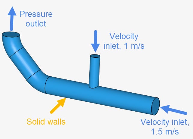
The base project is a simple internal pipe fluid simulation, with two inlets and one outlet. Find below, in Figure 1, an overview of the physics of the simulation:
To import the tutorial project, click on the button below:
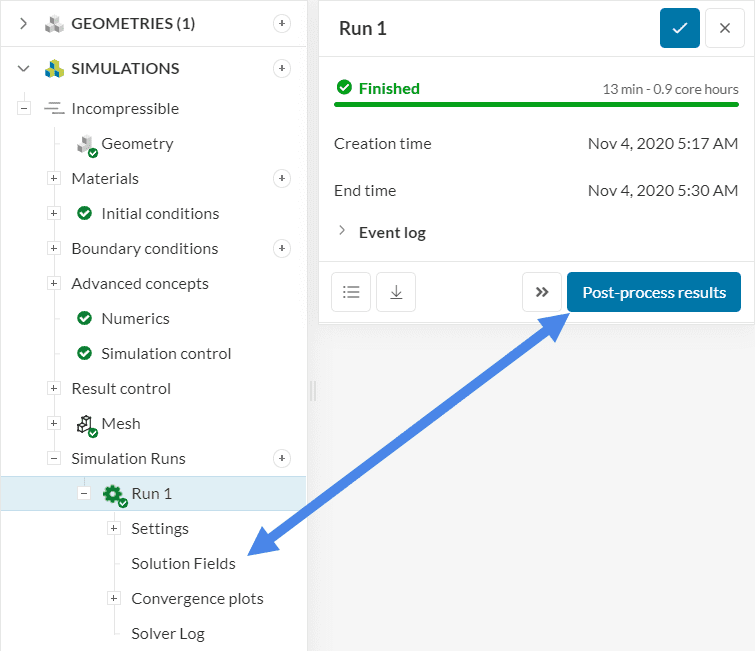
Firstly, when a simulation has results available, the run dialog box will prompt a ‘Post-process results’ button. Clicking this button or selecting ‘Solution Fields’ in the simulation tree will open the results in the online post-processor.
Note
The result will only load when you stay in the same tab where the Workbench is opened. The load time for the results will depend on the size of the data.
Introduction
SimScale’s post-processor interface is similar to the Workbench, keeping most of its functionalities. The post-processor also has general tools and filters that you can use to get the most out of your simulation results. To deeply understand all the features please refer to our standard document.
Legend Toggle
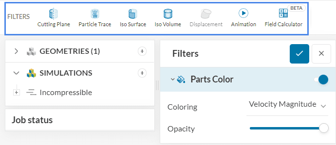
For this simulation, we are most interested in fluid velocity and pressure. Under Parts Color, you can select a parameter to plot on the boundaries of the model. Therefore, click on the dropdown and select ‘Velocity Magnitude’.
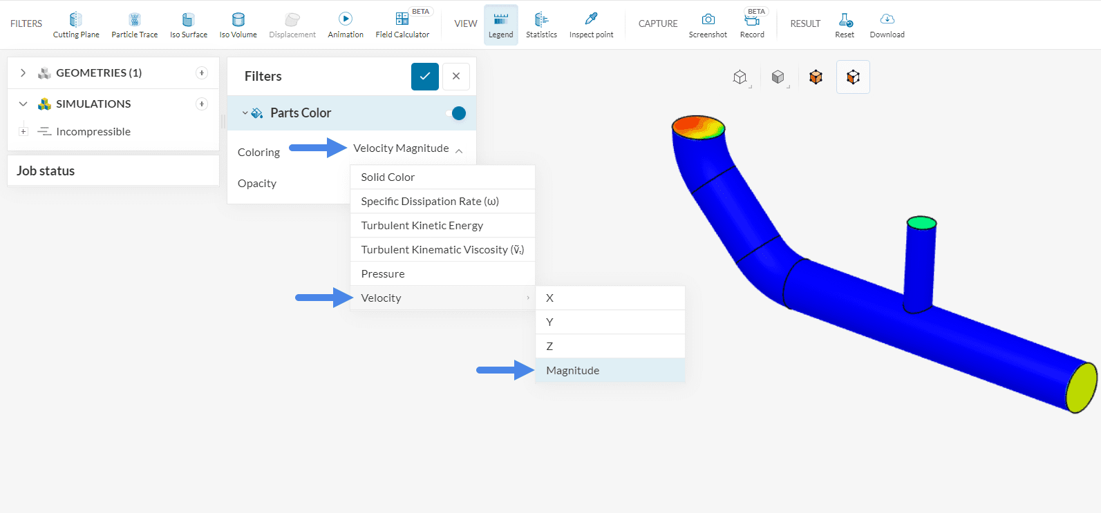
Through the legend, you can switch between quantities. All options shown in the image below can be edited:
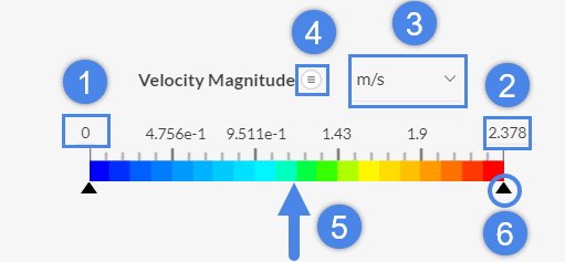
- Minimum scale range
- Maximum scale range
- Unit displayed
- Scalar/vector fields
- By right-clicking on the legend, you have access to a variety of options such as color schemes, data sets, automatic scaling, etc.
- The slider on the bottom is a quick way to adjust the scale range
Looking at figure 3, the outlet velocity is not uniform. To find out how the velocity varies at the outlet let’s use the Point inspection feature.
Note
Keep in mind the legend is only displayed when there are results selected. When no results or filters are selected, there is no legend visible.
Point Inspection
The Point inspection tool extracts a flow quantity at a certain location. To use the Point inspection tool, follow the steps below:
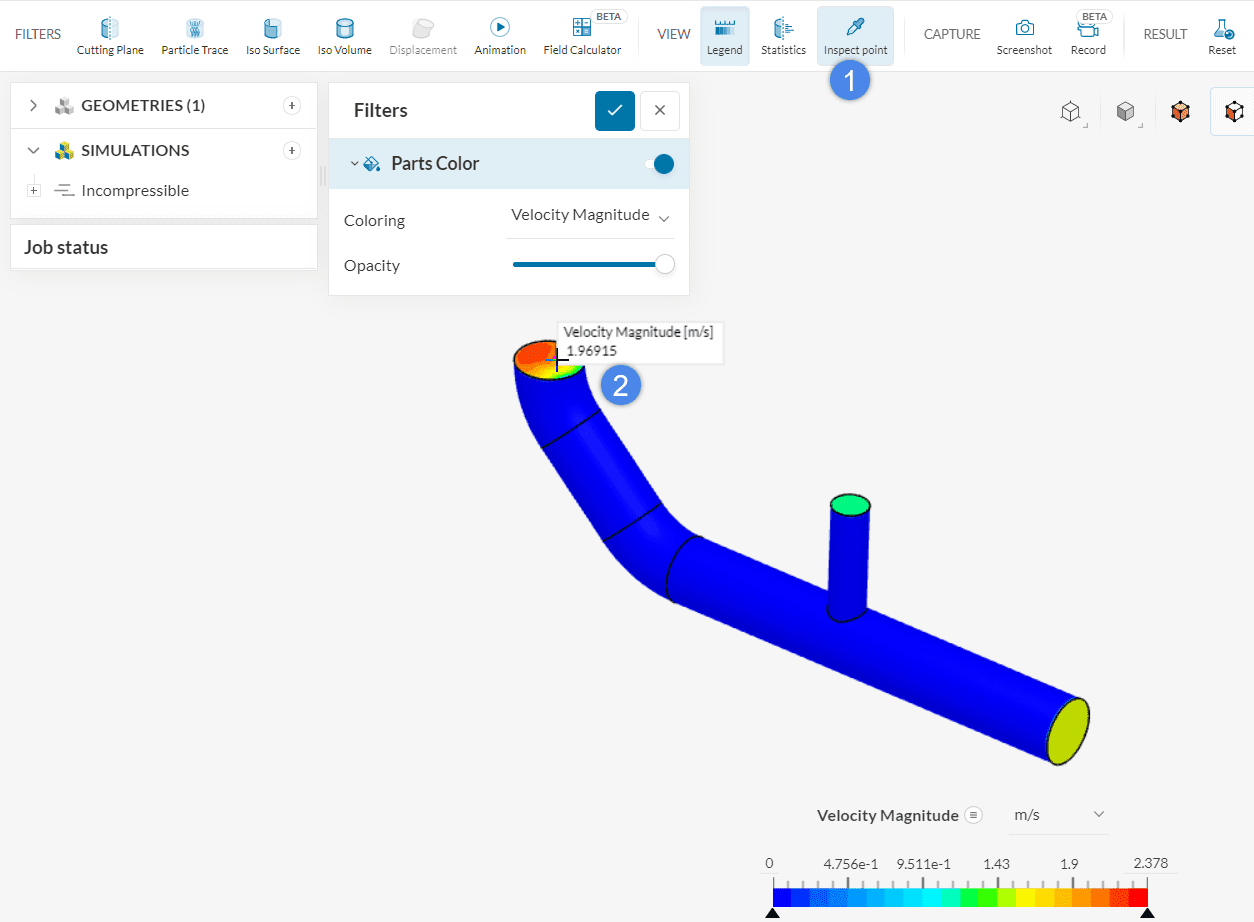
- Select the Point inspection
 tool in the post-processor.
 - Click on the point of interest to inspect the local results
By probing the velocity at the outlet, you will notice that it varies from approximately 0.4 to 2.2 \(m/s\). The variety in the outlet is caused by the shape of the pipe where it has a bend before the outlet. Now, we will try to get the average flow velocity at the outlet by using the Statistic feature.
Statistics
The Statistics feature shows additional values on a certain face or filter. Please follow the steps below to obtain the average velocity level on the outlet:
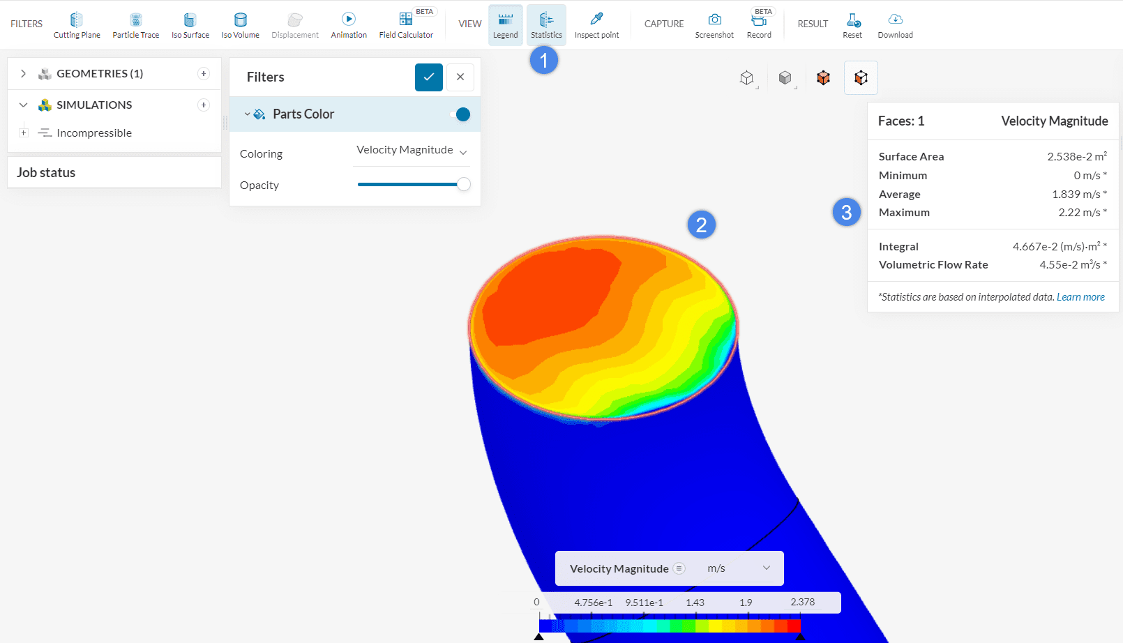
- Activate the ‘Statistics’ feature
- Select the face of interest
- A window opens up with a summary of the velocity values on the selected face
By using Statistics, not only can we get statistical values on the outlet but also the surface area of the outlet and the Volumetric Flow Rate. These values can be used to validate the simulation results of an experiment or hand calculations.
Screenshot
To create a screenshot, proceed as shown below:
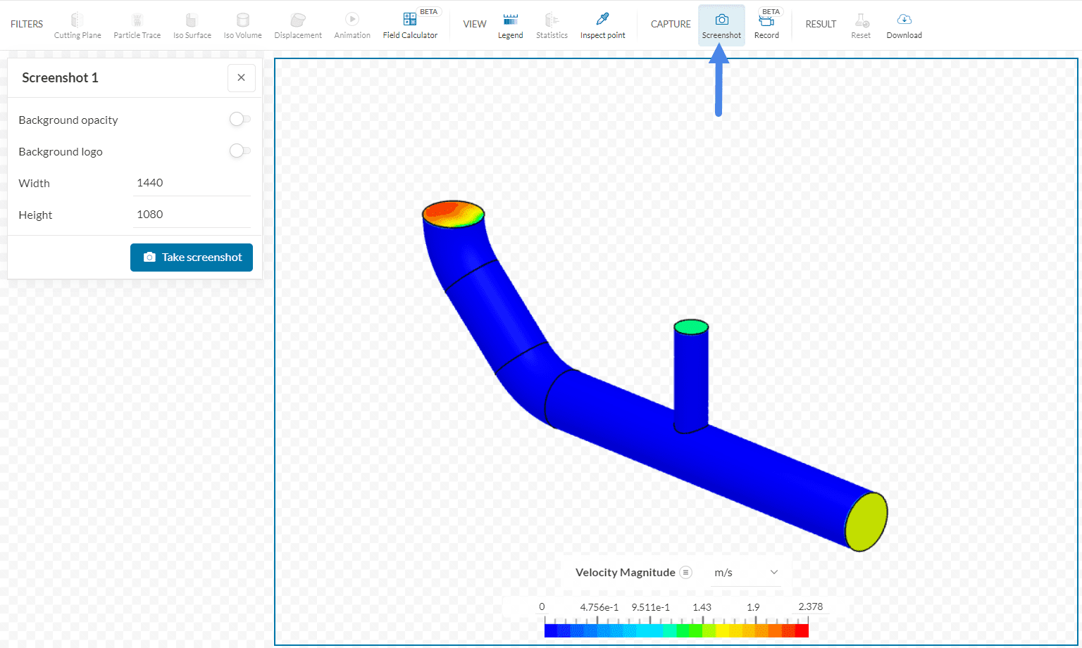
- Click on the camera icon

- A blue frame will appear, this is the area of the screenshot. This means the area or model of interest will need to be inside this frame. Click on ‘Take screenshot’ when ready.
After the screenshot is taken, you can change its name and provide a short description. The image can be downloaded or deleted in the screenshot dialog box.
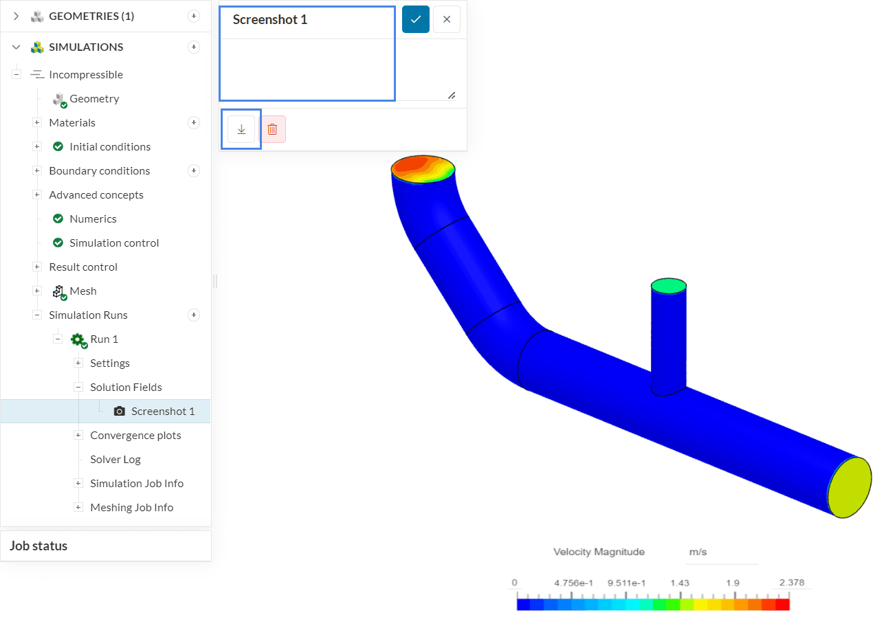
Note
The saved screenshots can be accessed again under Solution fields when you want to view or download them.
Filters
The Filters panel contains all the filtering tools we need to post-process the results.
Note
Filters can be combined with the coloring of the parts or with each other. Each filter will have its show/hide toggle.
Cutting Planes
Cutting planes or slices visualize a flow quantity on a particular cross-sectional area. Follow these steps to create a cutting plane:
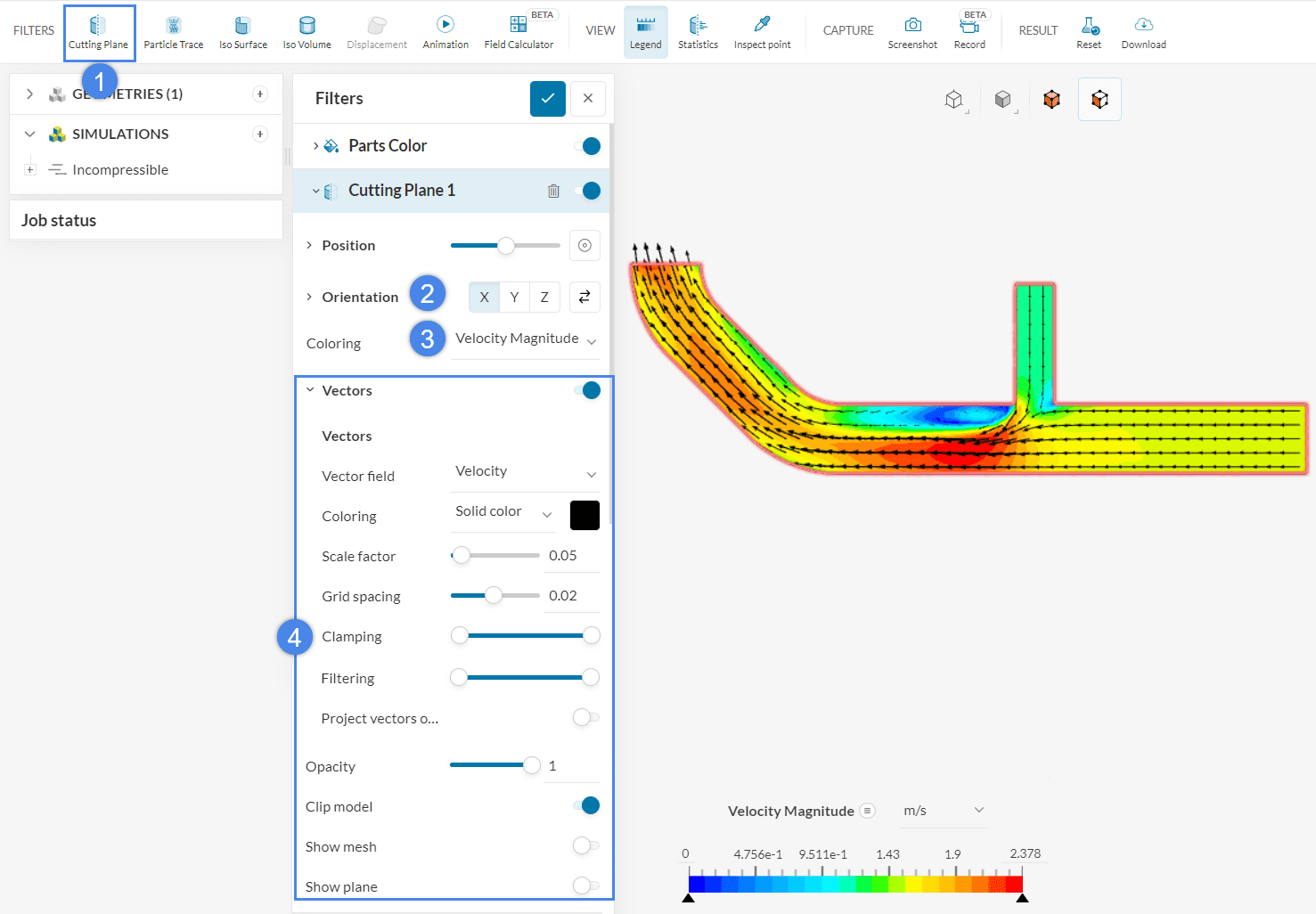
- Click on ‘Cutting Plane’ to create a new filter
- The Position of the plane will remain the same, but please adjust the Orientation to the ‘X’ axis
- Under Coloring, you can define which parameter to visualize
- With ‘Vectors’ toggled on, you will see a vector field representing the flow velocity. Vectors are highly customizable, allowing you to change their Color, Scale factor, Grid spacing, amongst other options
From figure 10, we can see that recirculation occurs near the junction area. This information will be important when redesigning the pipe to optimize the mixing.
Iso Surfaces
Iso Surface isolates regions in the model which match a given variable value. For example, if the user wants to know where the pressure is exactly 10 \(Pa\), Iso Surface is the choice. You can create an iso-surface by following the steps below:
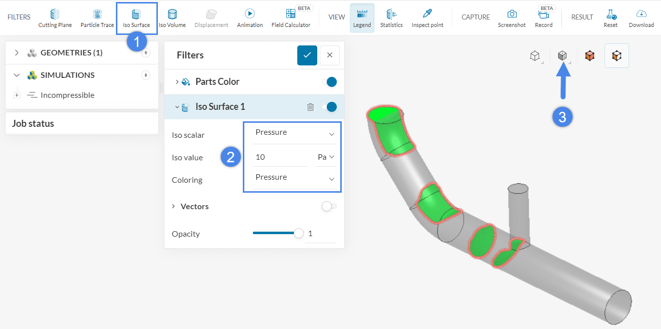
- Create a new ‘Iso Surface’ filter by using the top filter ribbon
- Adjust the Iso scalar to ‘Pressure’ with an Iso value of ’10’ \(Pa\). This will highlight the regions in the domain with a pressure of 10, Coloring them with ‘Pressure’
- You can adjust the Render mode to give you more perspective of the highlighted regions’ location
Iso Volumes
The Iso Volumes filter is very similar to Iso Surfaces, but instead of highlighting a single value, the Iso Volumes filter allows you to highlight a range. These are the steps to create iso volumes:
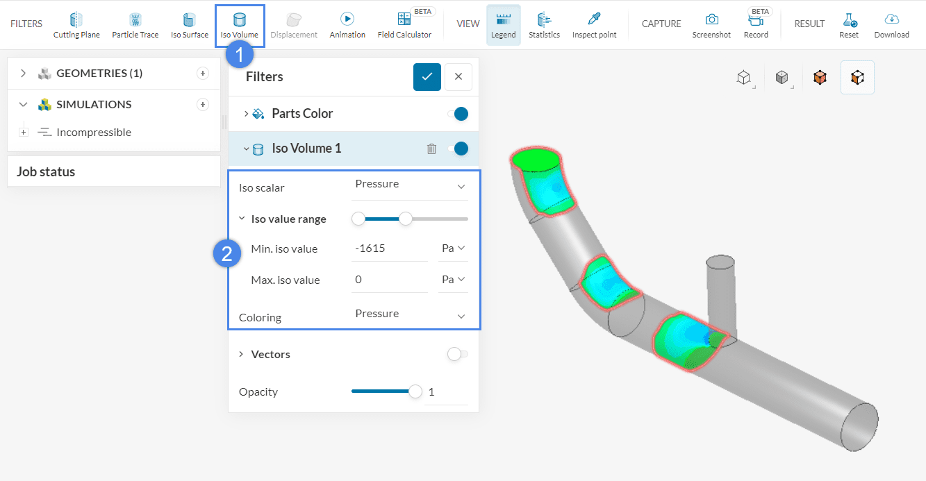
- Choose an ‘Iso Volume’ filter from the top ribbon
- In the configuration window, select ‘Pressure’ for the Iso scalar and set the Iso value range where the minimum is ‘-1615’ \(Pa\) and the maximum is ‘0’ \(Pa\).
Iso Volumes can help find regions where a quantity is over/below a certain threshold or requirement. From the figure above, we can see that the pressure reaches below 0 \(Pa\) around the junction, at the bend, and near the outlet. Similarly, Iso volumes can be used to isolate areas where cavitation occurs by changing the Max. iso value to the lowest allowable pressure before cavitation occurs.
Particle Traces
Particle Traces are similar to a dye that is injected into the flow and are often used to visualize the flow movement. Here are the steps to create Particle traces:
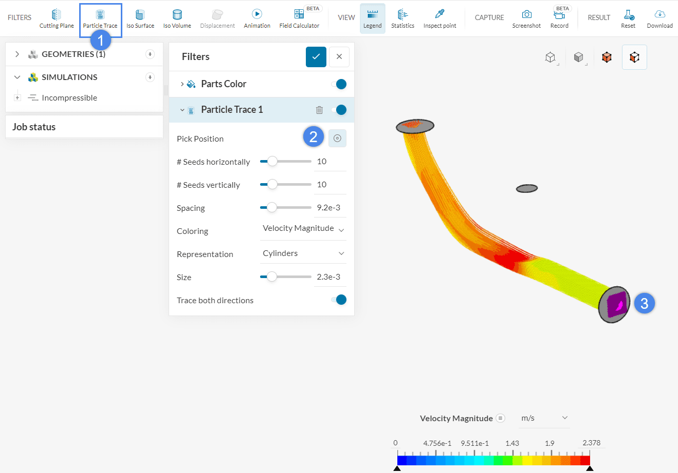
- Create a new ‘Particle Trace’ filter
- Make sure that the Pick Position icon
 is active. When it is on, you can click on a face to act as a seed face
 - Click on the main inlet face to place the seeds for the traces
Streamlines can be insightful in observing the fluid flow from a certain location – the seed face can either be defined on one of the faces of the model or on a cutting plane.
Animation
Once particle traces are generated, you can set them to move with an Animation filter:
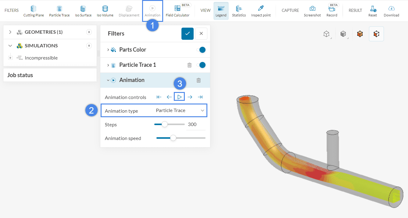
- Create a new ‘Animation’ filter
- Make sure to change the Animation type to ‘Particle Trace’
- Press the play button to start the animation
As a result, you will see how the traces evolve through the domain:
Congratulations! You have successfully finished the post-processing tutorial for the fluid flow simulation!
Note
If you have questions or suggestions, please reach out either via the forum or contact us directly.
Last updated: February 3rd, 2023
Did this article solve your issue?
How can we do better?
We appreciate and value your feedback.
What's Next
Tutorial: Post Processing Solid Mechanics Simulationpart of: SimScale Tutorials and User Guides


