Tutorial: Post Processing Solid Mechanics Simulation
In this article, we will demonstrate how the simulation results of the stress analysis of a connecting rod can be visualized and analyzed in your browser. This tutorial will also show SimScale’s post-processing environment capabilities. Import the finished project with the help of the button below:
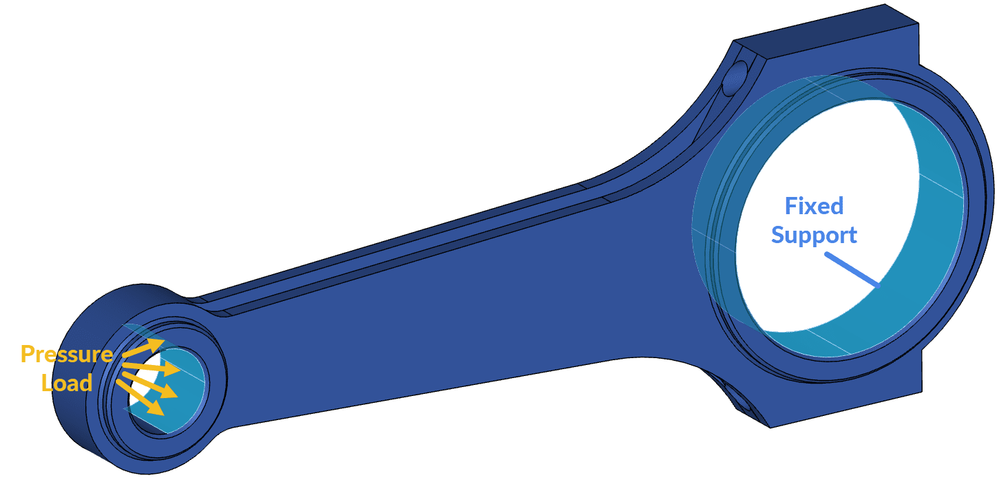
The base project is an engine piston connecting rod subject to a compressive load. Figure 1 below shows the boundary conditions for the simulation:
1. Accessing the Online Post-Processor
After the simulation run is successfully completed, the computed results are available to be analysed using the online post-processor. To open it, you can use one of two methods:
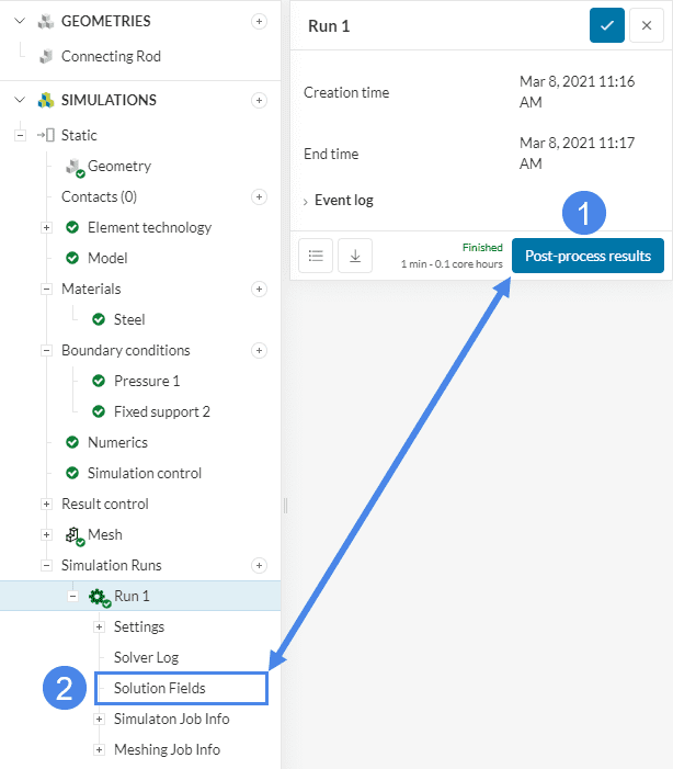
- Use the ‘Post-process results’ button from the simulation run dialog.
- Select the ‘Solution Fields’ tree item under the completed simulation run.
This takes you directly to the online post-processor with the simulation results loaded and ready to create some visualizations.
2. Visualizing Stress
Upon loading the online post-processor, you will notice that the connecting rod is already colored by default. In order to find out exactly what you are looking at, you can check the Filters panel at the top left:
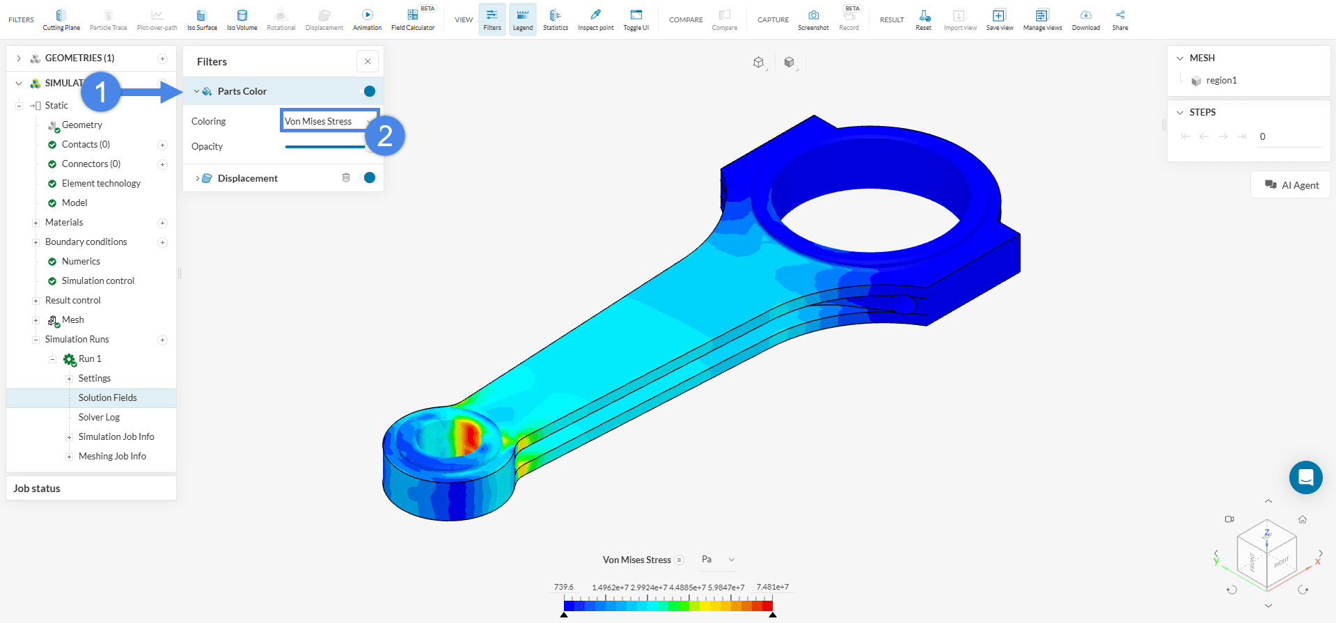
From the Filters panel, expand the section ‘Parts Color’ to see that the connecting rod is colored by the Von Mises Stress by default. If your results display a different field, please go ahead and select Von Mises Stress.
You should see a plot similar to the one shown in Figure 4 below. We will also show a few ways to tweak this plot and make it better:
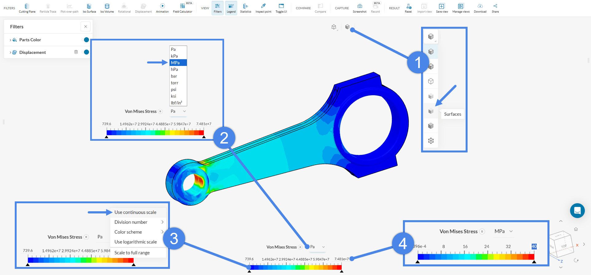
- Set the render mode to ‘Surfaces’.
- Set the field units to ‘\(MPa\)’.
- Right-click the legend bar and select ‘Use continuous scale’.
- Keep legend maximum value to ’40’.
Our final stress plot can be appreciated after applying the tweaks:
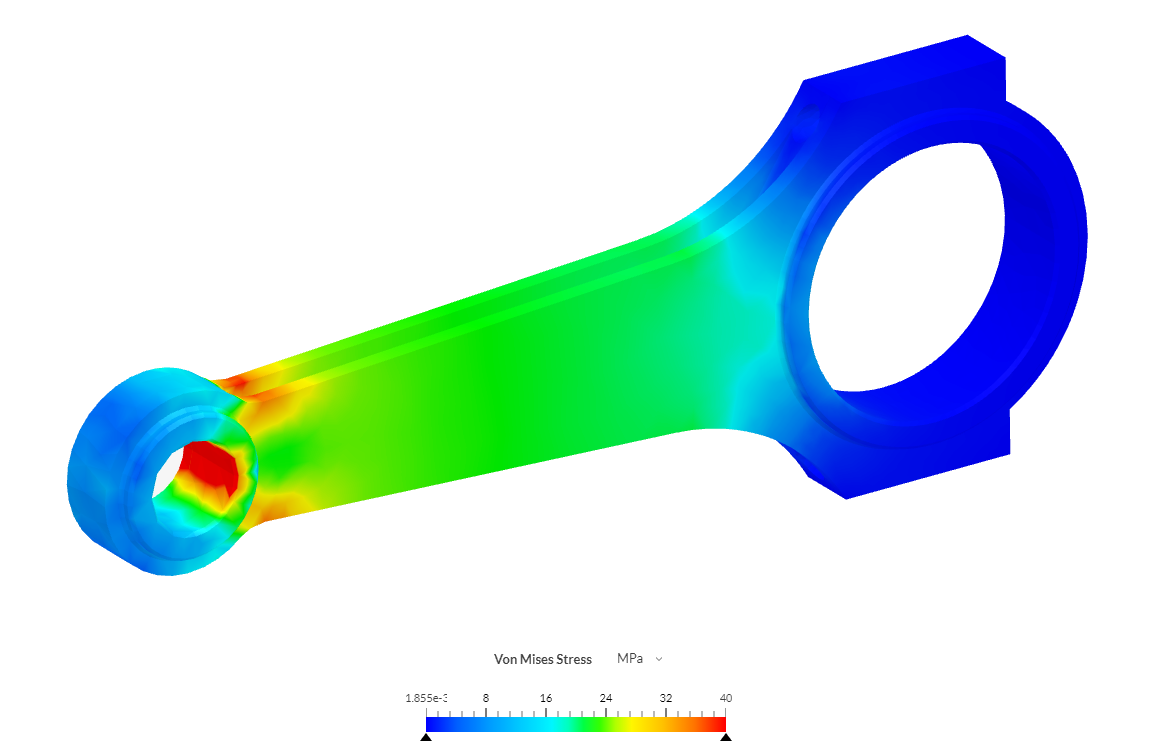
It can be seen that the maximum stress values appear close to the region of application of the compressive load, and that some additional stresses are developed behind the reinforcing ring around the shaft connection hole (left). No significant stresses are developed in the region of the fixed support.
3. Visualizing Deformation
In order to see the effect of the loading on the shape of the connecting rod, we can create a deformation plot. For this, a Displacement filter is added by default to the Post-processor:
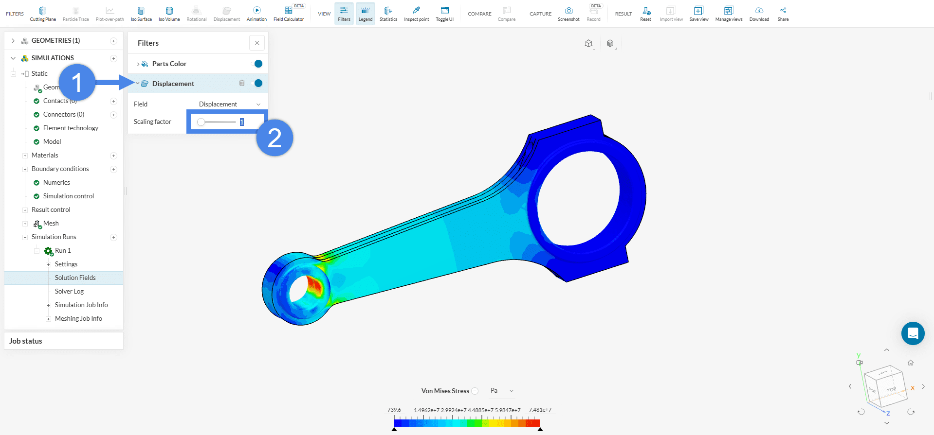
At a Scaling factor of 1, the deformation is not apparent as you can see. Thus, in order to properly visualize the deformed shape, please set the Scaling factor to 500.
Then, we can also change the color legend to find out the value for the displacement, by clicking on the legend field:
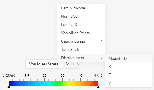
After this, please also apply ‘Use continuous scale’ option for the color legend, just as we did for the stress plot.
You should end up with a plot such as the one shown in Figure 8 below:
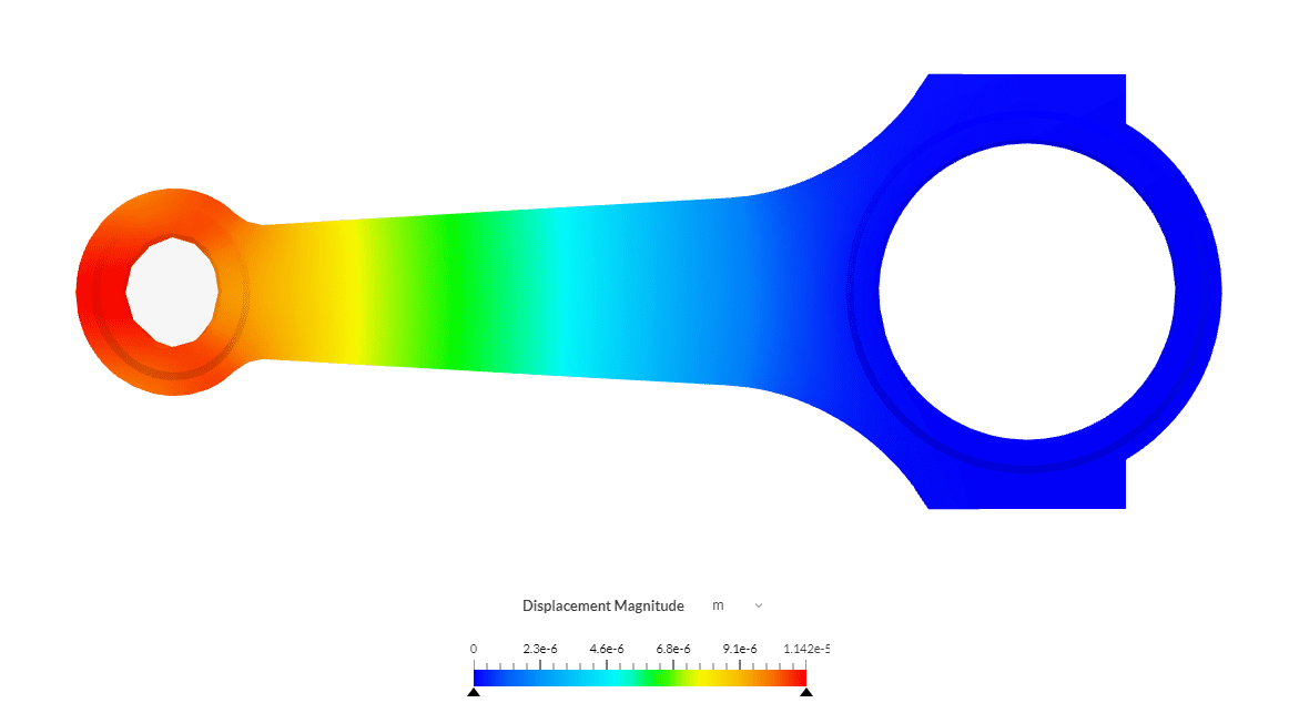
It can be seen that the highest deformation is located at the end of the connecting rod, with a displacement magnitude of 1.14e-5 \(m\), in the axial compressive direction.
4. Animating the Results
An animation for the deformation of the rod can help us better visualize the loading process. It can be created by adding an Animation filter using the ‘Add Filter’ button from the Filters panel.
The default Animation type of Time Step is adequate for transient simulations, but for our static analysis we have to perform some changes:
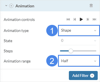
- Set the Animation type to ‘Shape’.
- Set the Animation range to ‘Half’.
Now you can press the ‘Play’ button to start the animation:
Animation 1 displays the axial compression of the connecting rod. The deformation process shows the effects of length reduction, the lateral expansion of the small end, and the ovalization of the hole, with a maximum displacement of 1.1e-5 \(m\).
5. Further Steps
You can now continue analyzing the dataset: For example, you can visualize more fields, coloring the part by strains, or by applying additional filters such as isosurfaces and isovolumes.
If you need additional details on how to control the online post-processor, you can have a look at our post-processing guideline.
6. Perform a Complete Simulation
In case you are interested in setting up the connecting rod simulation from the beginning here is the tutorial link that will help you with the setup as well as the post-processing:
Last updated: July 29th, 2025
Did this article solve your issue?
How can we do better?
We appreciate and value your feedback.


