Tutorial: Electromagnetics Simulation on a Magnetic Lifting Machine
This tutorial showcases how to use SimScale to run an electromagnetics simulation on a Magnetic Lifting Machine.
Overview
This tutorial teaches how to:
- Setup and run an electromagnetics simulation;
- Create external flow region ;
- Assign multiple materials, and other properties to the simulation;
- Mesh with the automatic standard meshing algorithm.
We are following the typical SimScale workflow:
- Prepare the CAD model for the simulation;
- Set up the simulation;
- Create the mesh;
- Run the simulation and analyze the results.
1. Prepare the CAD Model and Select the Analysis Type
To begin, click on the button below. It will copy the tutorial project containing the geometry into your Workbench.
The following picture demonstrates what is visible after importing the tutorial project.
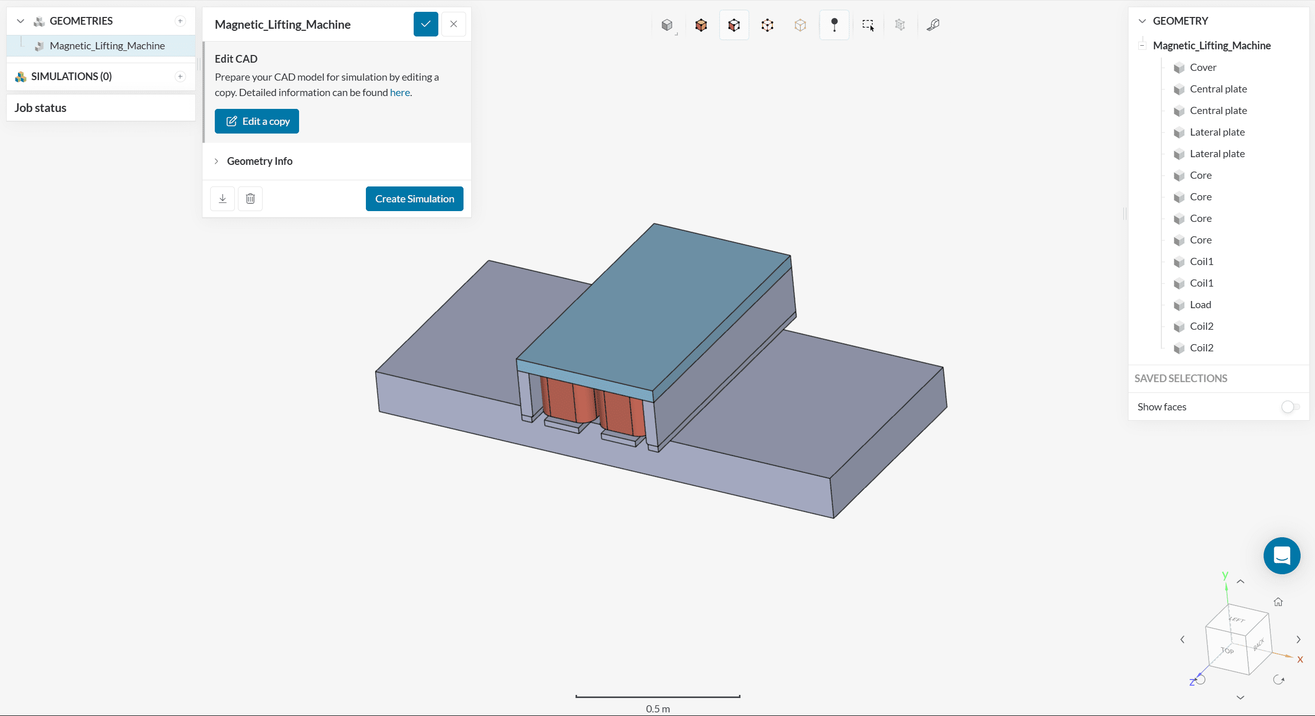
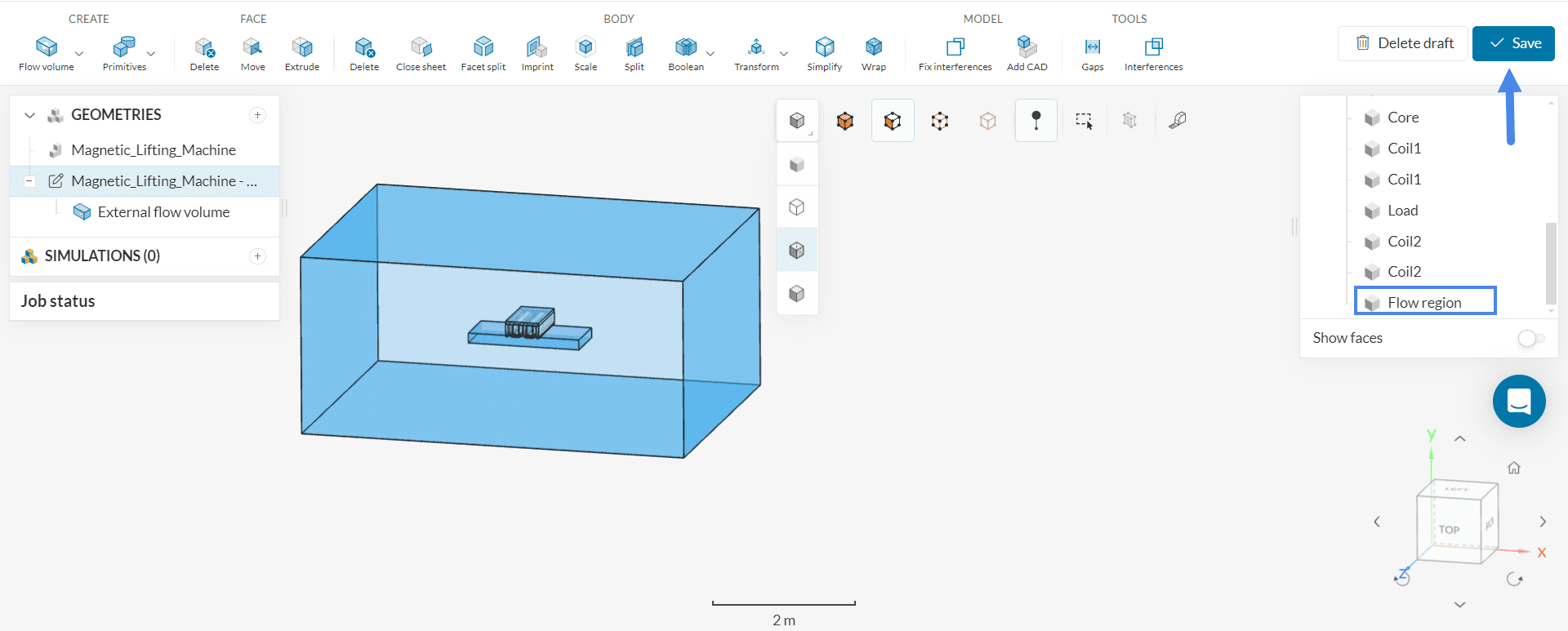
The geometry consists of an actual Magnetic Lifting Machine. It consists of multiple parts as can be observed in the scene tree.
1.1 Geometry Preparation
The geometry for this tutorial is not ready for electromagnetic simulations. It contains multiple solid parts of the assembly, but not a flow region. A flow region is necessary for Electromagnetics simulations because it controls where the fields are calculated.
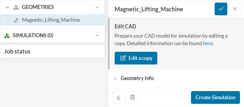
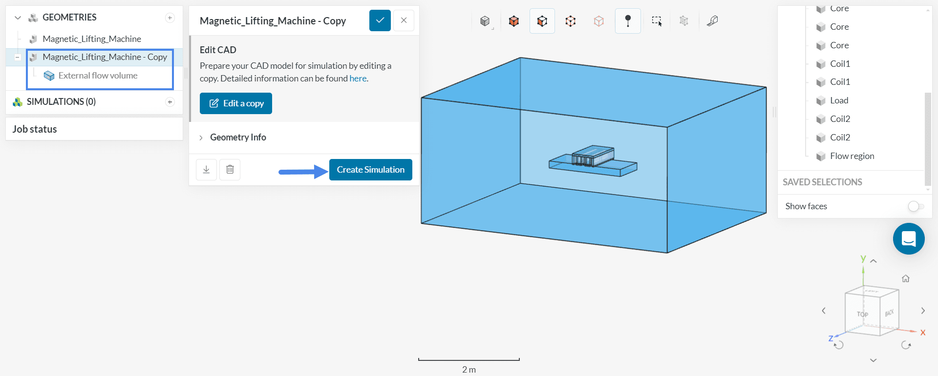
To create a flow volume click on the ‘Edit a copy’ button. This will allow to perform modifications on the copy of the already existing CAD.
Now perform the following steps:
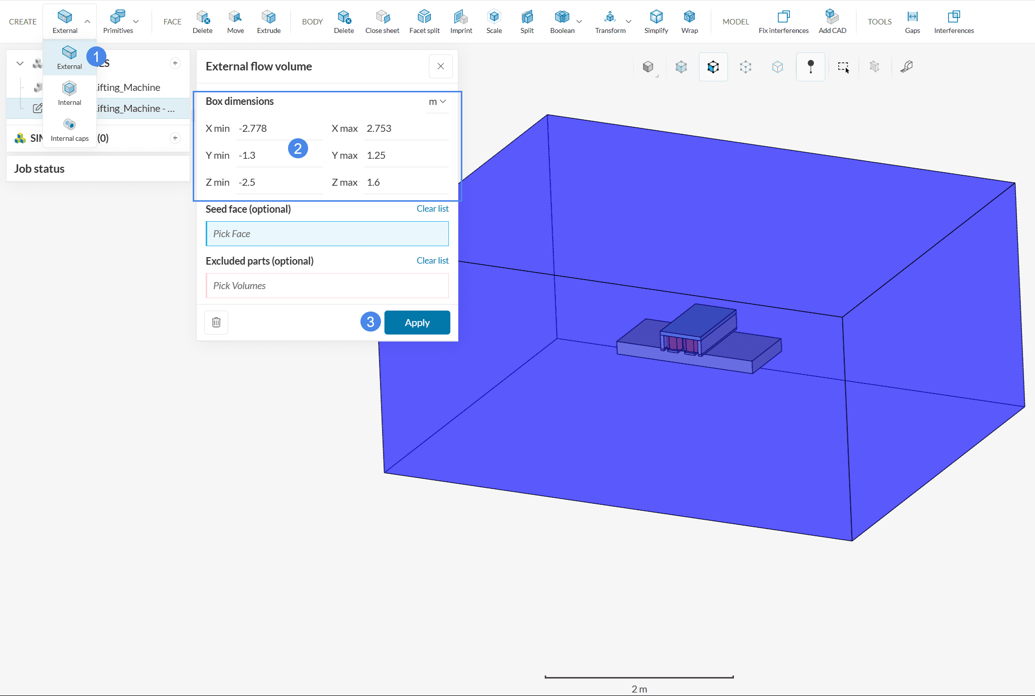
- Select the ‘External Flow Volume operation’. This will lead to a settings panel where the user needs to define the box dimensions. It is important that the boundaries of the flow region are far from the region of interest, so that they do not interfere with results around the solid parts. Once the minimum and maximum dimensions are defined, click ‘Apply’.
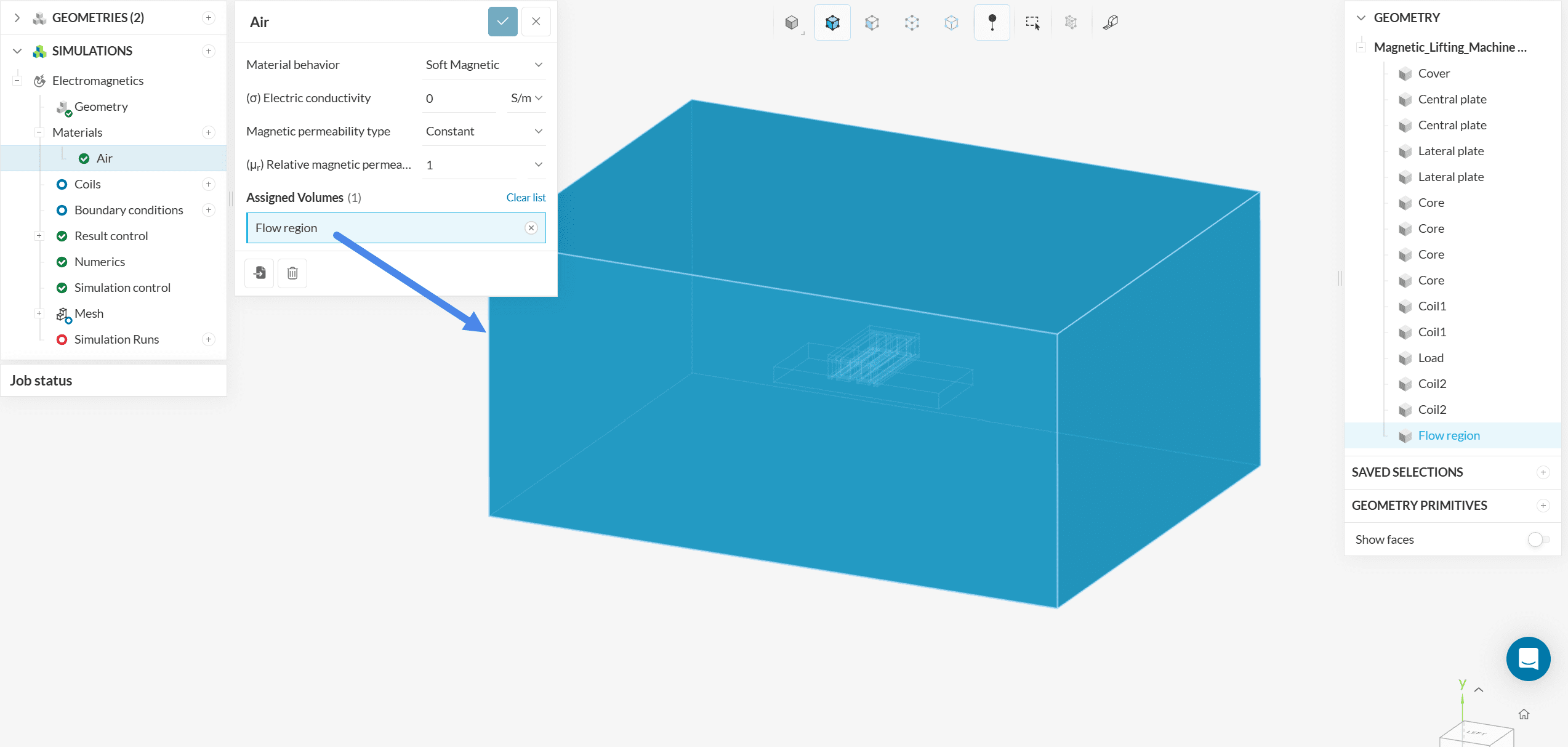
Notice that there is a new volume entity called Flow region under the parts list at the very end (see Figure 5). Use the ‘Save’ button to bring this new geometry back to the Workbench.
The modified geometry (with the Flow region) will appear under Geometries as a copy of the original valve geometry.
1.2 Create the Simulation
Click on the new geometry ‘Magnetic Lifting Machine – Copy’ and hit the ‘Create Simulation’ button. You can rename it if you’d like.
This will open the simulation type selection widget:
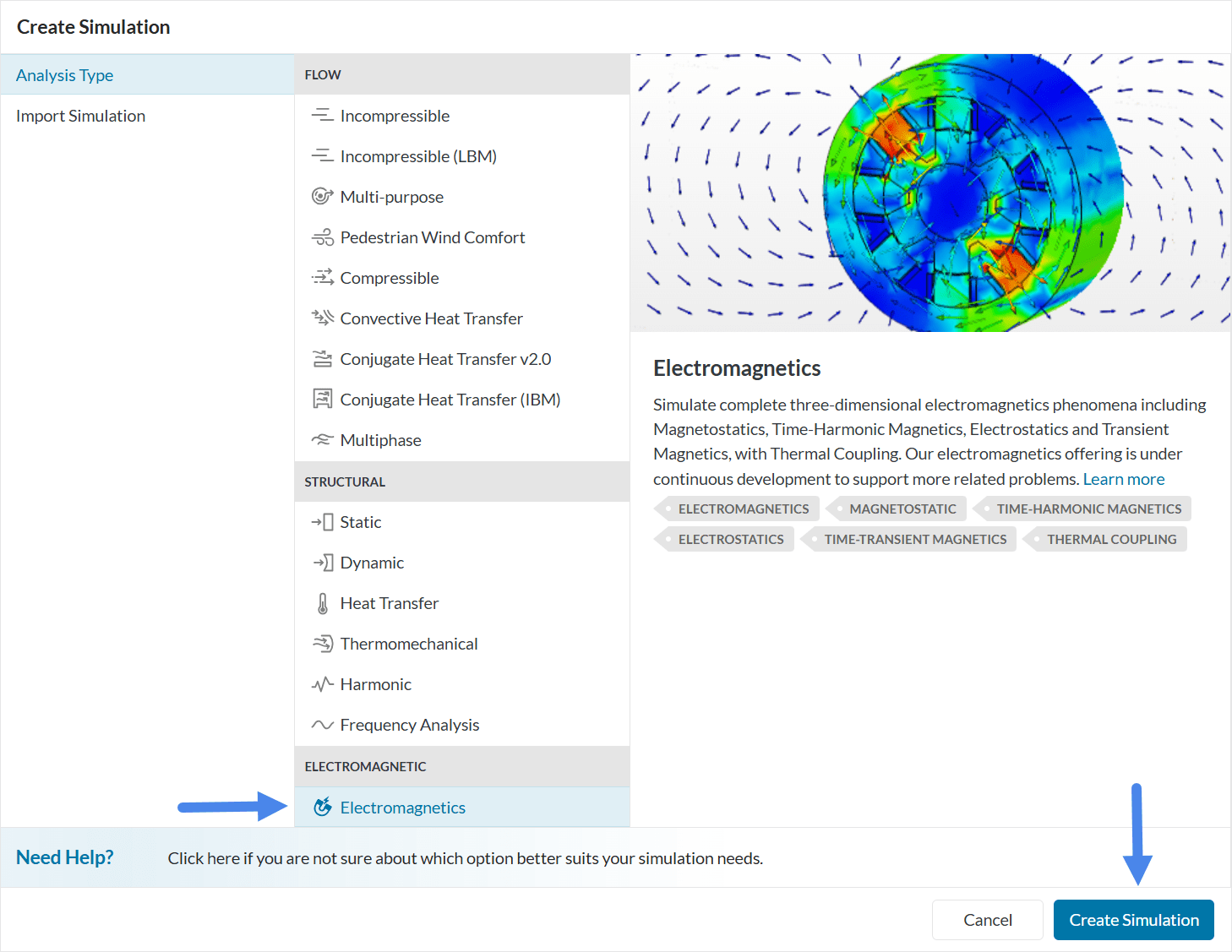
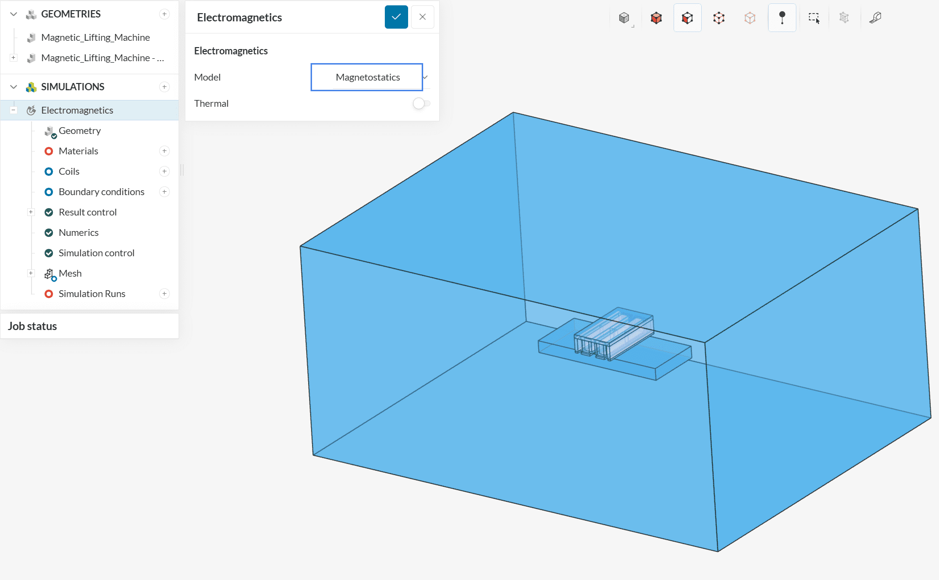
Choose ‘Electromagnetics‘ as the analysis type and ‘Create Simulation’. Since we are dealing with time-constant magnetic fields this tutorial will be solved under the Magnetostatics model.
At this point, the simulation tree will be visible in the left-hand side panel.
2. Pre-Processing: Setting up the Simulation
2.1 Define Materials
This simulation will begin with air initially present in the flow region. Then we will assign Copper, Steel, and AISI 1008 Steel to the solid bodies. Therefore, this simulation will use four materials. Hence, click on the ‘+ button’ next to Materials. In doing so, the SimScale fluid material library opens, as shown in the figure below:
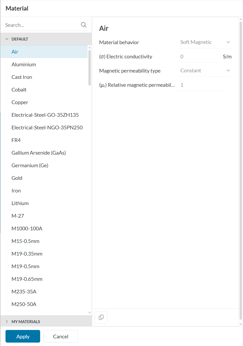
Select ‘Air‘ and click ‘Apply’. This means air will be recognized by the flow region throughout the simulation. Keep the default values, and assign the entire Flow region to it (if not already by default).
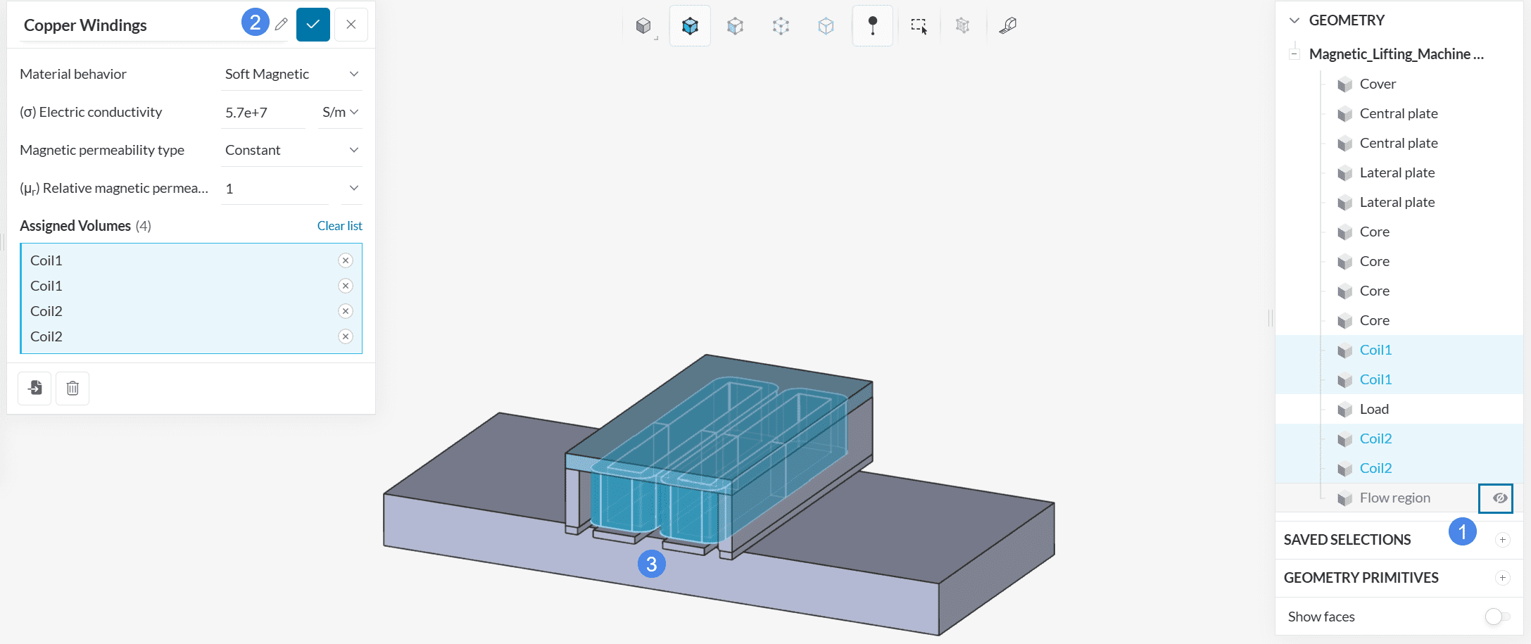
Repeat the same procedure for the material Copper and assign it to the coils. We can rename the material to ‘Copper Windings’. To view the solid parts, hide the Flow region and select the coils as shown in Figure 11.
Repeat the procedure for Steel and assign it to Load as shown in Figure 12. Please note that the flow region is still hidden. We can rename the material to ‘Typical Steel – Workpiece’.
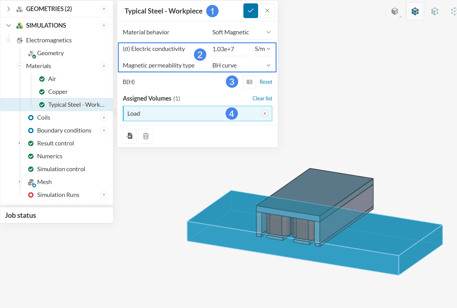
Change the material properties, namely Electric conductivity to 1.03e+7 \(S/m\) and Magnetic permeability type to ‘BH curve’. We then need to set B(H). For this, we use a table. Download the CSV file ‘B(H)_Typical Steel’ below and upload it to your project.
Repeat the procedure once again for Steel, assign it to 9 volumes as shown below, and rename it to ‘AISI 1008 Steel – Core’.
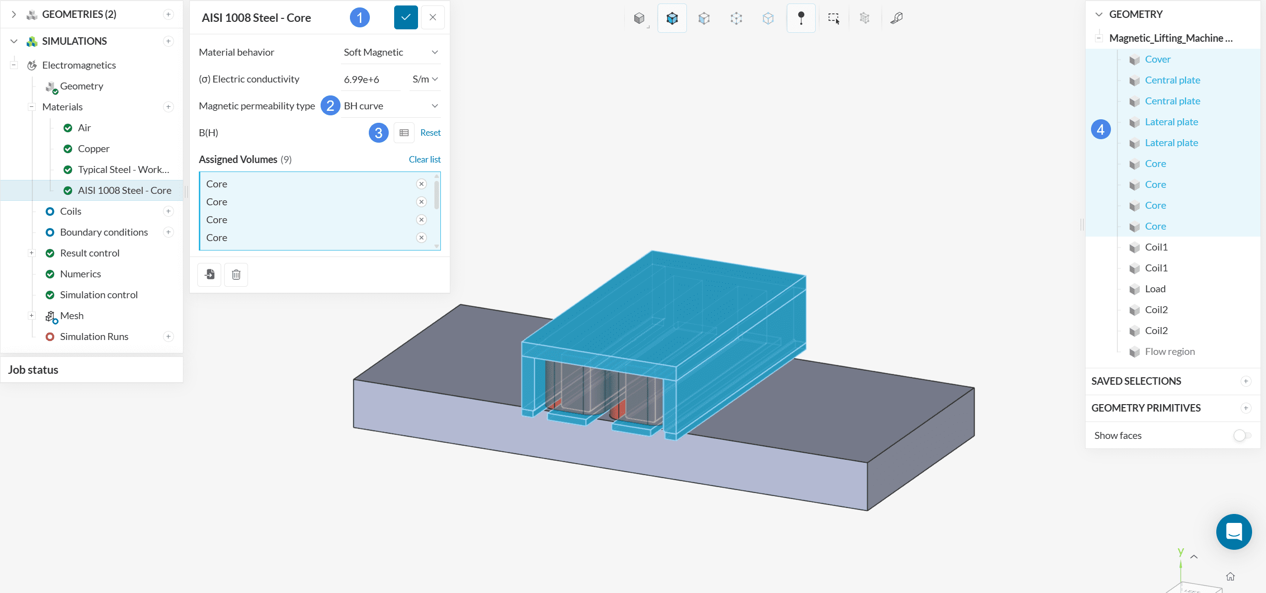
Keeping the value for Electric conductivity as default, change the material property Magnetic permeability type to ‘BH curve’. Now upload a CSV file for B(H) by downloading the ‘BH_1008Steel’ file attached below.
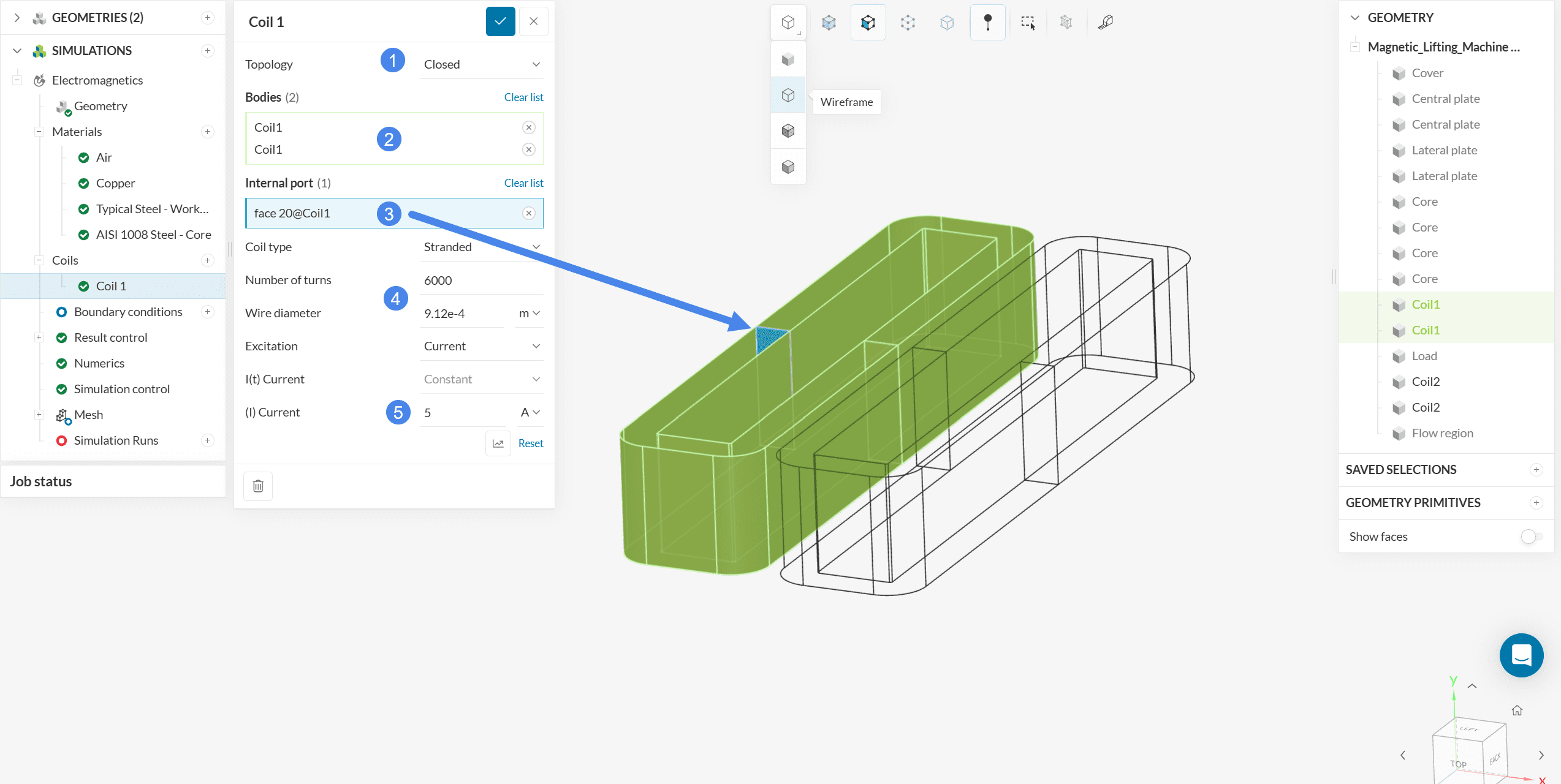
2.2 Assign the Coils
Under Coils in the simulation tree, we will assign two coils named ‘Coil 1’ and ‘Coil 2’. Please select the faces and change the respective values as shown in Figure 14 and Figure 15 (shown in Wireframe mode for ease). Hide all other volumes and the outer surfaces until the inner face of the coil is visible. To hide faces, select them and right-click to select the ‘Hide selection’ option from the drop-down. Continue until you see the face as shown in both figures. Please make sure to change the values for Topology, Number of turns, Wire diameters, and (I) Current.
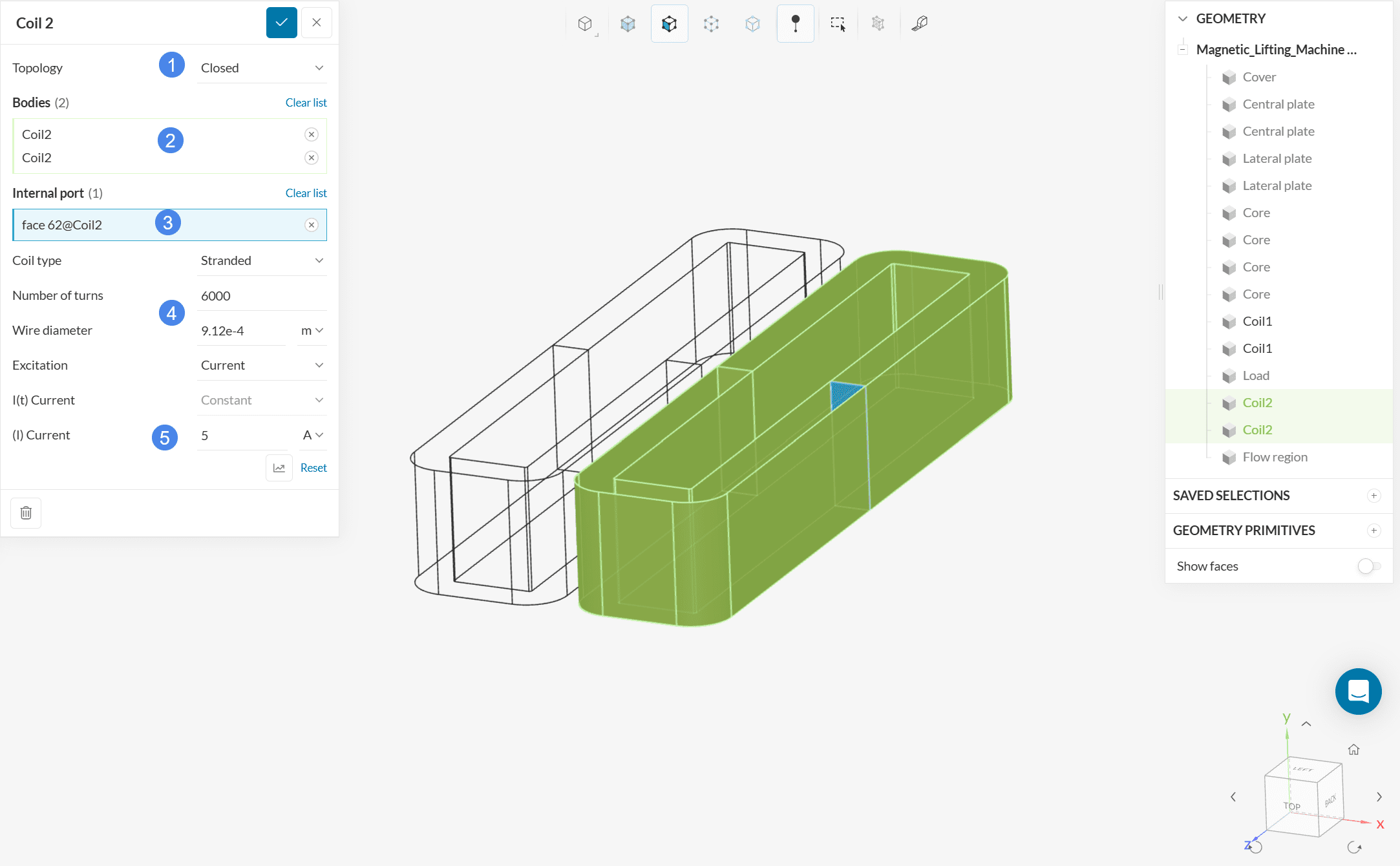
Repeat the procedure for ‘Coil 2’ as shown in Figure 15.
2.3 Assign the Boundary Conditions
There are no boundary conditions for this simulation.
2.4 Result Control
Result control allows you to observe the convergence behavior globally as well as at specific locations in the model during the calculation process. Hence, it is an important indicator of the simulation quality and the reliability of the results. Remember to toggle on ‘Calculate Inductances’ under Result control.
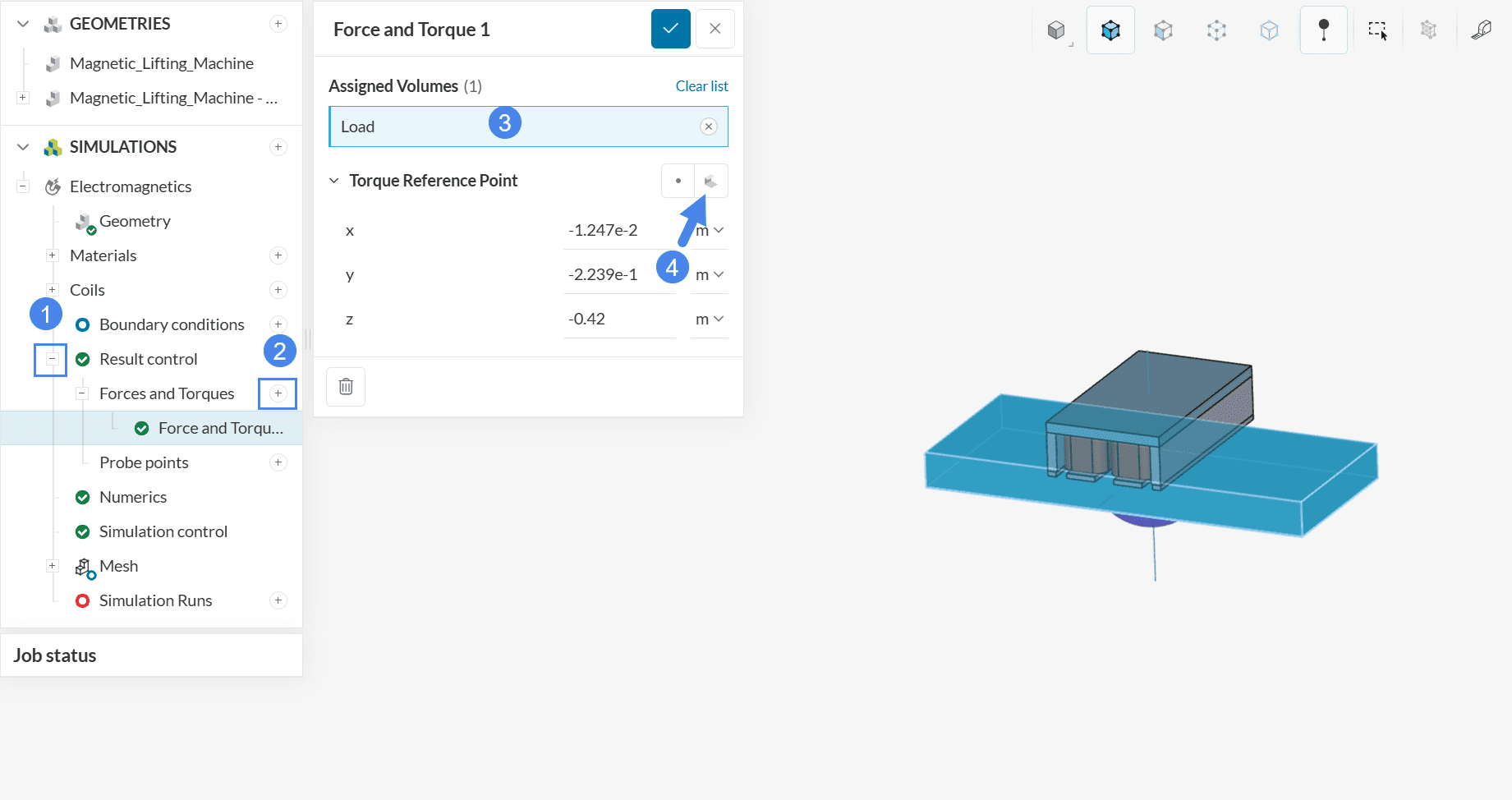
a. Forces and Torques
For this simulation, set a ‘Forces and torques’ control on the Load of the valve. Click on the ‘+’ icon under Result control> Forces and torques to open the settings panel. After assigning the load volume to the forces and torques result control, you can either type in the coordinates for the Torque Reference Point, or use the Pick center of current selection button (highlighted by the blue arrow) to input the coordinates from the figure below:
2.5 Numerics and Simulation Control
The Numerics and Simulation control for this simulation, are optimised with their default values and need not be altered.
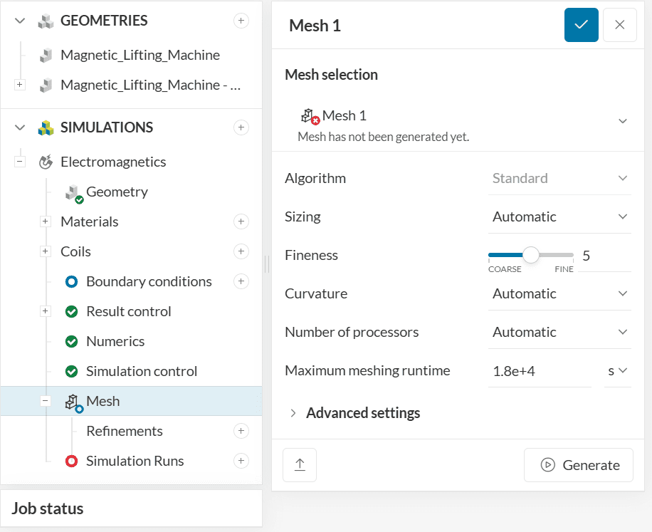
3. Mesh
To create the mesh, we recommend using the Automatic mesh algorithm, which is a good choice in general as it is quite automated and delivers good results for most geometries.
In this tutorial, a mesh fineness level of 5 will be used. If you wish to undertake a mesh refinement study, you can increase the fineness of the mesh by sliding the Fineness slider to higher refinement levels or using the region refinements.
Did you know?
The automesher creates a body-fitted mesh which captures most regions of interest using physics based meshing.
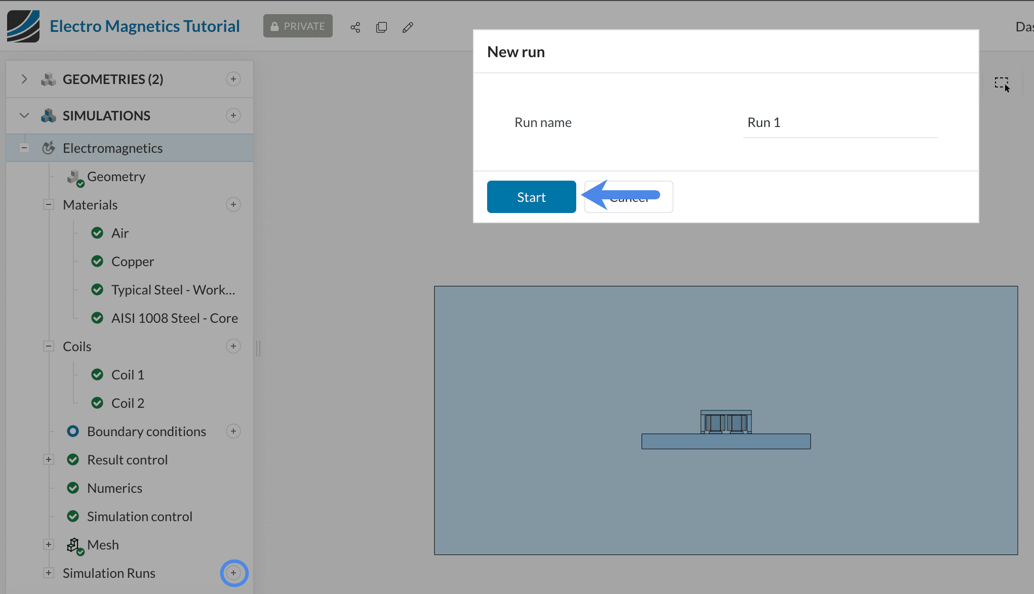
4. Start the Simulation
Now you can start the simulation. Click on the ‘+’ icon next to Simulation runs. This opens up a dialogue box where you can name your run and ‘Start’ the simulation.
While the results are being calculated you can already have a look at the intermediate results in the post-processor by clicking on ‘Solution Fields’ or ‘Post-process results’. They are being updated in real-time!
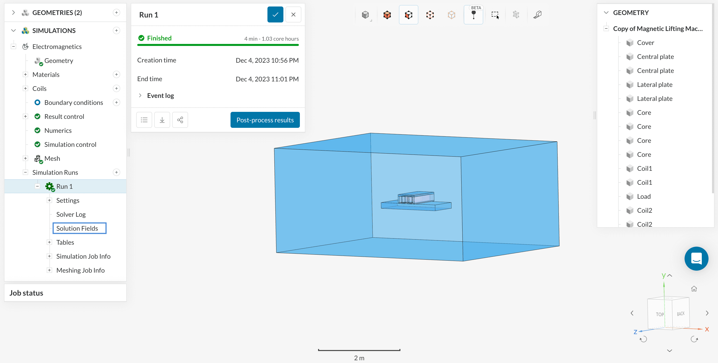
Depending on the instance chosen by the machine, it might take 5-10 minutes for the simulation to finish. Once finished access the online post-processor as indicated in Figure 19.
5. Post-Processing
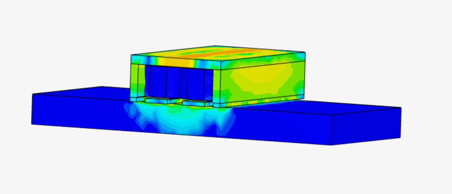
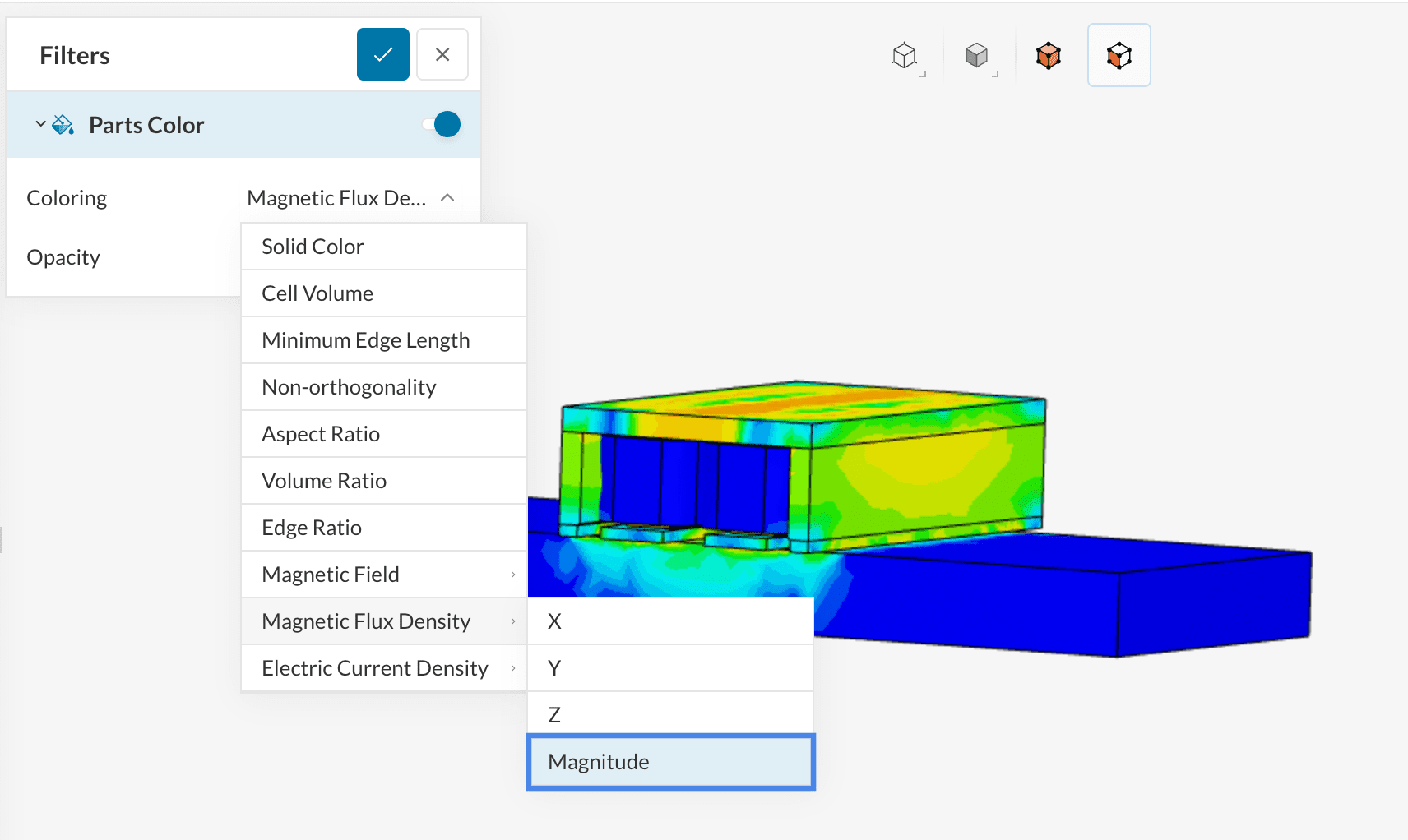
5.1 Magnetic Flux Density Magnitude
Once inside the post-processor, under the Parts Color filter change Coloring to ‘Magnetic Flux Density Magnitude’.
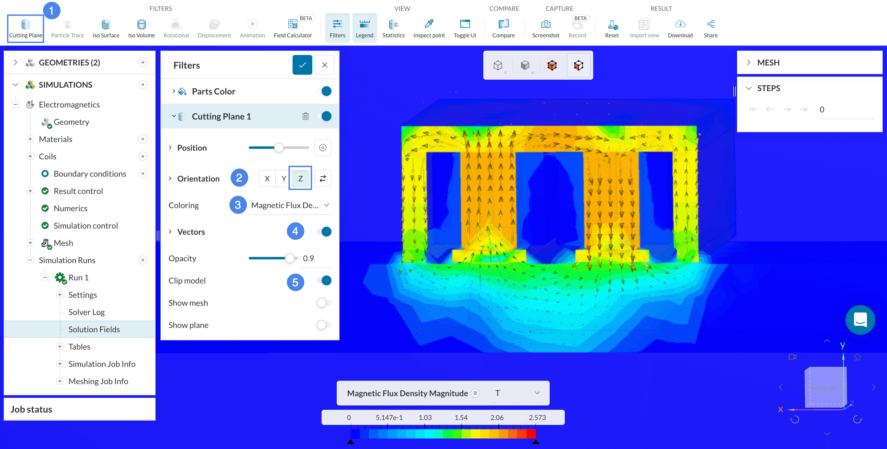
- Hit the ‘Cutting Plane’ filter from the top ribbon.
- Adjust the position accordingly and set the orientation of the plane to ‘Z’ axis.
- Adjust Coloring to represent the magnetic flux density magnitude
- Toggle on Vectors to visualize the magnetic flux flow direction.
- Toggle on Clip model so that the cut plane view can be visible.
After a few seconds, you will see a clip showing the inside of your model.
Different parameters can be viewed by changing the coloring. In this tutorial, we will have a look at Electric Current Density Magnitude and Magnetic Field Magnitude as well.
5.2 Electric Current Density Magnitude
To view the Electric Current Density Magnitude, follow the steps below:
- Create a ‘Cutting plane’ filter using the top ribbon.
- Adjust the Orientation of the cutting plane to the ‘Y’ direction.
- Set the Coloring of the plane to ‘Electric Current Density Magnitude’
- Toggle on Vectors and choose the vector field as ‘Electric Current Density Magnitude’
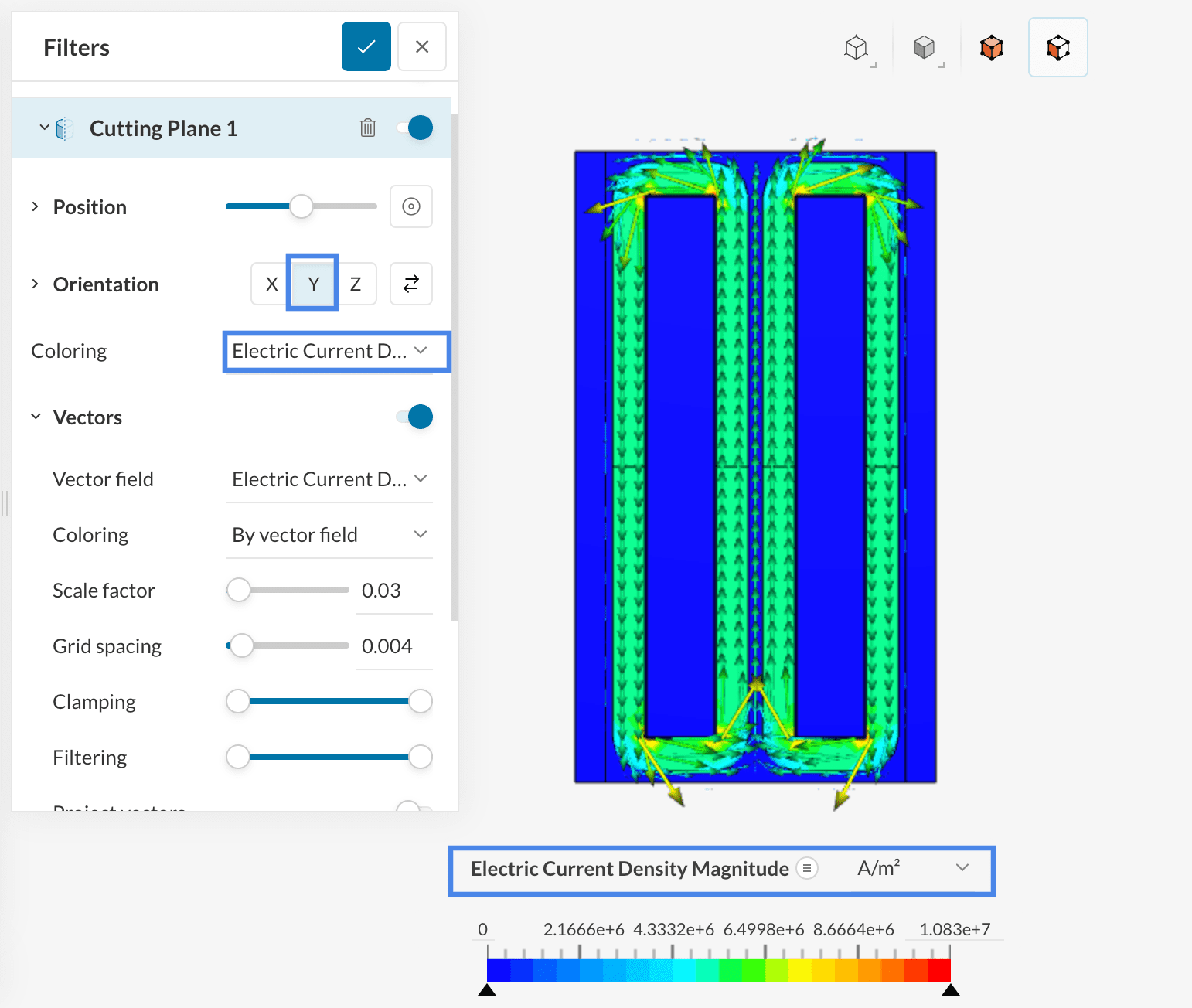
From Figure 22, you can see the strength and direction of the current flow. Thicker, closely packed lines denote higher current densities, while thinner, more spaced-out lines signify lower densities. The direction of the lines illustrates the path a positive charge would take. The continuous nature of these lines indicates the uninterrupted flow of current.
5.3 Magnetic Field Magnitude
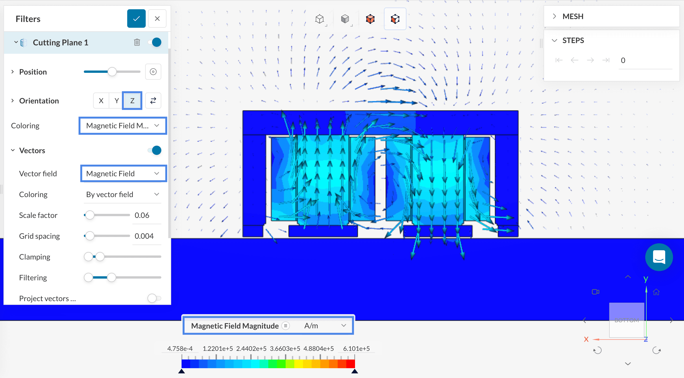
- Create a ‘Cutting plane’ filter using the top ribbon.
- Adjust the Orientation of the cutting plane to the ‘Z’ direction.
- Set the Coloring of the plane to ‘Magnetic Field Magnitude’.
- Toggle on Vectors and choose the vector field as ‘Magnetic Field Magnitude’
From Figure 23, you can see the magnetic field arrows which represent both the strength and direction of the magnetic field. Longer, closely spaced arrows indicate a stronger, more concentrated field, while shorter, sparser arrows denote a weaker field. The direction of the arrows signifies the path a north pole would follow, from the north pole of the magnet to its south pole, forming closed loops that reveal the continuous nature of magnetic fields.
5.4 Forces and Torques on the Load
The Forces and Torques results are of particular interest in the simulation. The load will be subjected to forces and torques as assigned and we can also view the resistances and inductances on both the coils Coil 1 and Coil 2. Hence, let’s inspect the results in the tables:
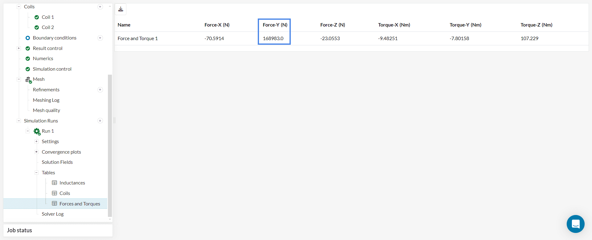
Numerical Noise
Since the value of interest is the force in the \(\mathrm{Y}\) direction, only it is relevant to the analysis and the other components might vary as a result of numerical noise (they should be close to 0 due to the problem’s symmetry).
Analyze your results further with the SimScale post-processor. Have a look at our post-processing guide to learn how to use the post-processor.
Note
If you have questions or suggestions, please reach out either via the forum or contact us directly.
Last updated: April 7th, 2025
Did this article solve your issue?
How can we do better?
We appreciate and value your feedback.


