This article explains why parts collide in nonlinear static analysis and the methods to prevent this.
Solution
Short answer: If parts collide, one of the following happened:
- There was no physical contact defined between the parts: Ensure that all the contacts are correctly defined.
- The penalty coefficient is too low: Increase the penalty coefficient and simulate again. Do this until the penetration depth is negligible.
Please visit the documentation page to learn more about the Static Analysis type. In addition, you will find more detailed info about Nonlinear Contacts, Penalty Contact and Lagrangian Contact on this page.
General Tips to Prevent Colliding Parts
Important information
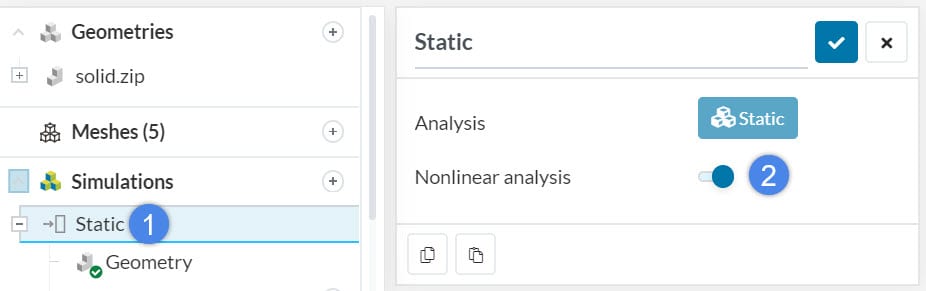
If multiple parts could touch during the simulation, you must enable Nonlinear analysis in Static analysis type. This will allow you to assign Physical contacts.
Assign Physical Contacts Correctly
Physical touching of parts is modeled using physical contacts. They should be defined by:
- the faces, that are already in contact
- the faces, that are going to interact during the nonlinear study
Important information
Before starting a nonlinear static analysis with multiple bodies in physical contact, imprint the geometry. Check this knowledge base article to see what imprint does to your model.
Let’s take a look and see how a physical contact is assigned properly:
In the following simple example, you see a quarter model of small and large cylinders:
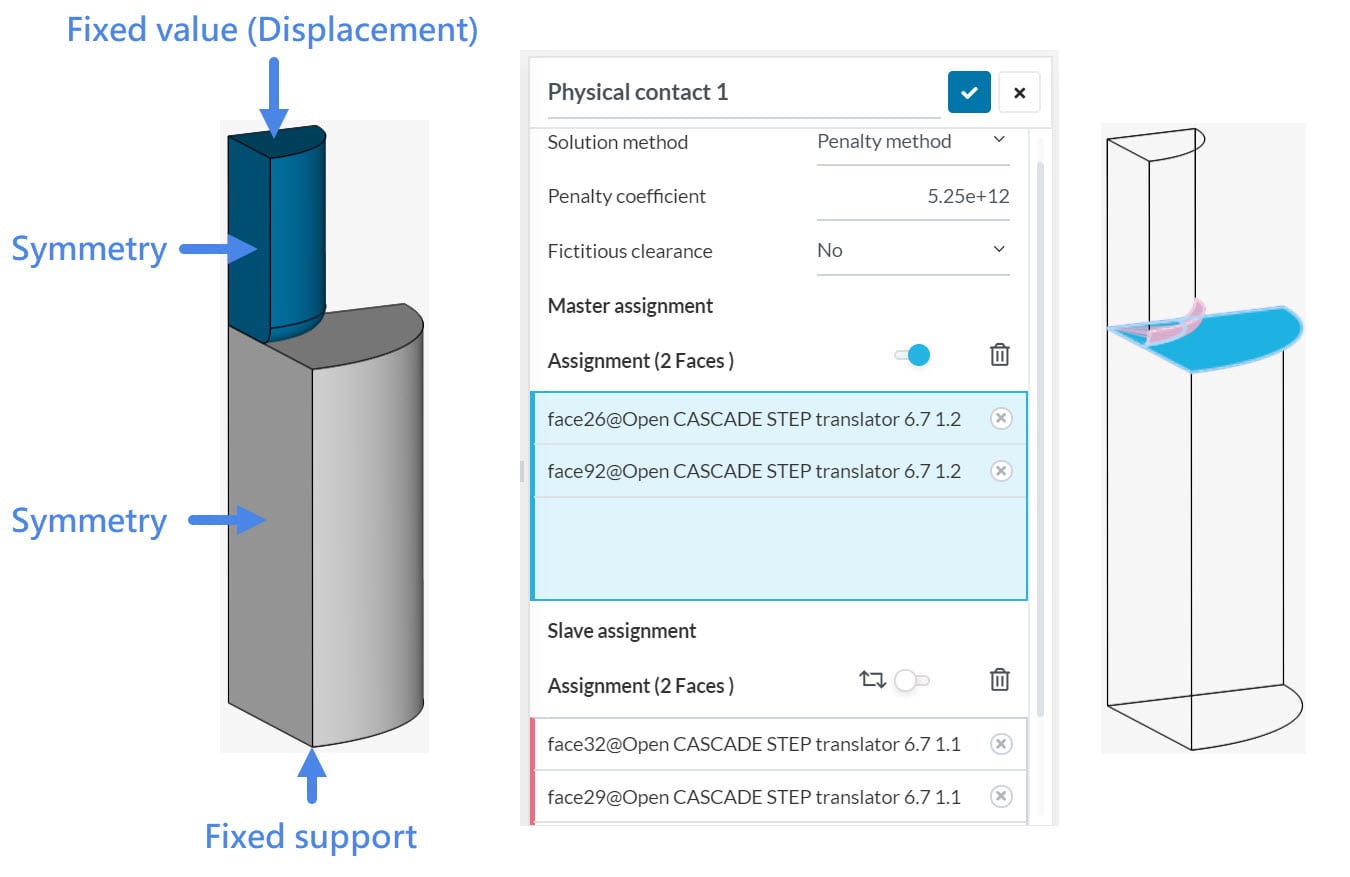
- We want to find out the force required to create a specific displacement on the smaller body.
- Therefore, we apply a displacement and measure the Nodal Force.
- We model the contact properties between the small and large bodies by using a physical contact.
Now we need to define which surface is the master and which the slave. If you are wondering how to choose, this knowledge base article gives recommendations about which surfaces should be chosen as master and which as a slave.
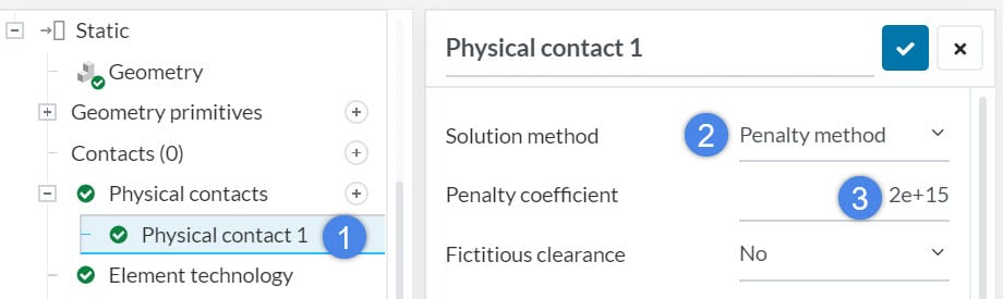
In SimScale, there are two methods for modeling physical contacts and avoid situations in which parts collide:
- Augmented Lagrange Method
- Penalty Method
Each method has it’s own advantages and disadvantages.
Penalty Method
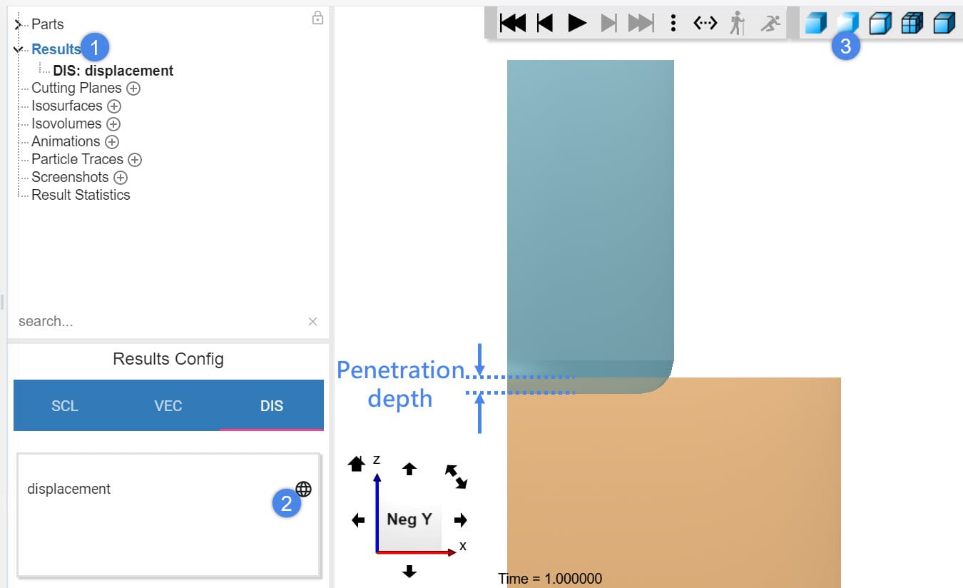
- The penalty method is based on the assumption that two bodies collide (overlap) and an imaginary spring is compressed during the collision.
- The amount of collision is called penetration depth.
- The contact force is then calculated with respect to the penetration depth and stiffness coefficient of the spring.
- The penalty coefficient is the stiffness of the contact (imaginary spring).
$$F = k \cdot \Delta L $$
Where, \(k\) is the stiffness of the contact (Penalty coefficient), \(F\) is the contact force, and \(DeltaL\) is the penetration depth.
- Estimate k (penalty coefficient) and perform an initial simulation
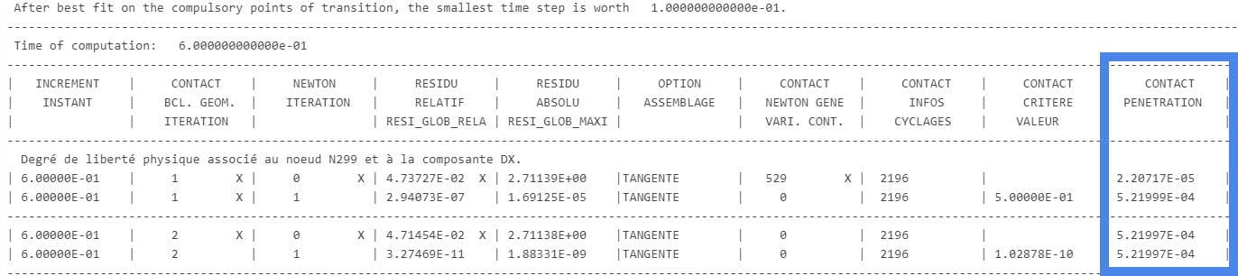
- Check the solver log. Are the Contact penetration residuals small enough? A good threshold might be 1e-6.
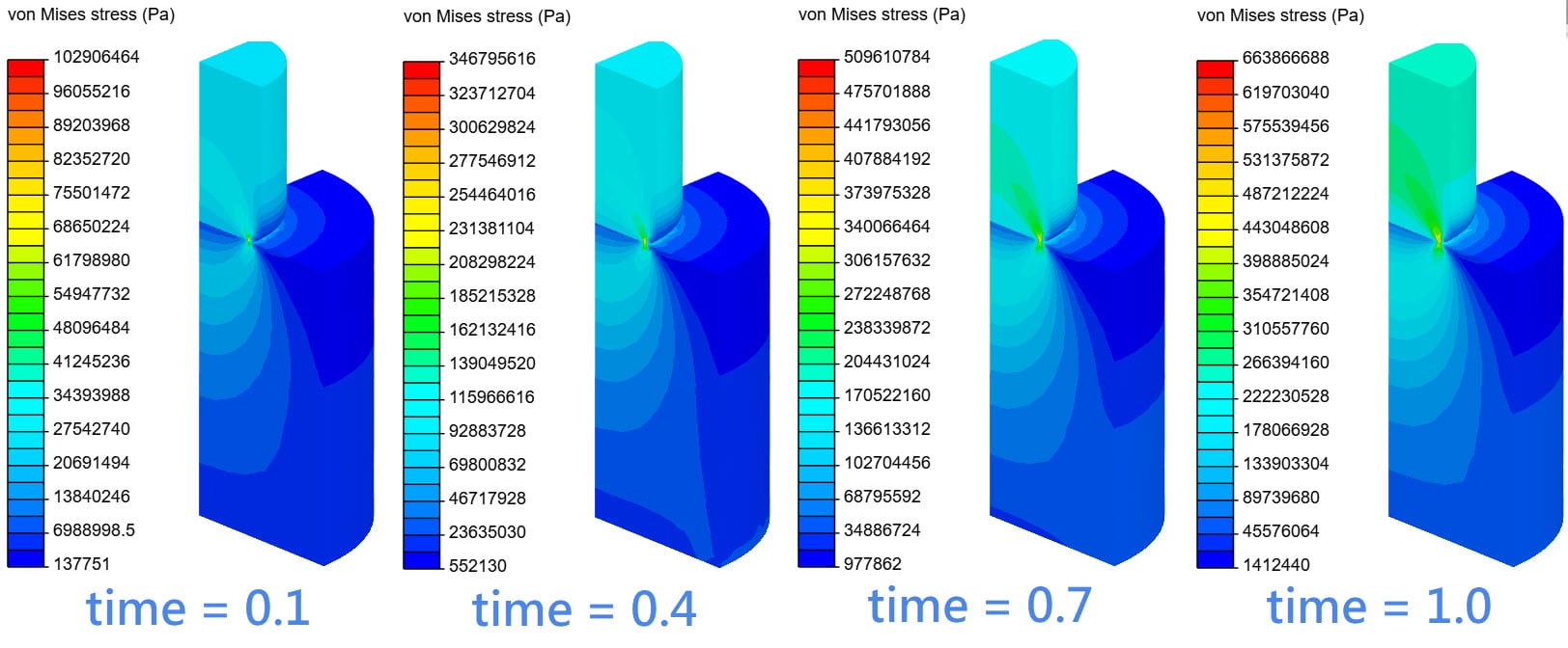
- If the contact penetration is small enough, check the solution fields. View displacement results and check the penetration. Is the penetration negligible?
- If penetration residual or penetration depth is large, then increase the k. If the simulation fails (The solution matrix is singular error), then better decrease the k. To tune the k, multiply it with by the factor of 10, 100, or 0.1, 0.01.
- As a rule of thumb, you can multiply the Young’s modulus by 50 [1]
$$k = 50 \cdot E $$
where, \(E\) is the Young’s modulus. - G.R. Liu recommends to multiply the Young’s modulus by a factor of 1e5 or 1e8 [2]
$$k = 1 \cdot 10^{5 \sim 8} \cdot E $$ - In Code_aster documentation, it is recommended to multiply the largest Young’s modulus of the bodies in contact by a characteristic length [3]
$$k = d \cdot E_{max} $$
where, \(d\) is the characteristic length. - Zienkiewicz recommends to use the following equation [4]
$$k = E_{max} \cdot (\frac{1}{d})^p $$
The characteristic length can be defined as the ratio of the element size to the dimension of the problem domain.
$$d = \frac{\Delta x}{n} $$
where, \(d\) is the characteristic length, \(p\) is the order of elements, \(Delta x\) is the element size (nodal spacing) of the smallest element in contact face, and \(n\) is the dimension of the problem domain (SimScale requires 3D domain, therefore n = 3)
In the penalty method, it is important to assign a suitable penalty coefficient. A suitable penalty coefficient should keep the penetration depth at a minimum:
If it’s too small, then bodies will overlap.
If it’s too big, it will generate numerical instabilities.
A good practice is to do the following:
Determination of the Penalty Coefficient
The penetration coefficient depends on many factors, such as mesh type, element size on contact surfaces, material properties, load, etc. There is not any particular way to define the penalty coefficient. However, you can use one of the following recommendations. The complexity increases from top to bottom:
Augmented Lagrange Method
In contrast to the Penalty coefficient, penetration is completely forbidden in the Lagrange method.
Thus, the contact force is independent from cell size. This method requires an exact solution (Lagrange equations) instead of iterations, which makes it accurate but unstable in large deformations.
The Augmented Lagrange method can be considered as a combination of Penalty and Lagrange methods. It causes minimal penetration and solution is almost exact. This method is accurate, but not suitable for problems with more than 100,000 nodes. It is also less stable, especially with second order elements.
Best Practices:
- The Penalty method is recommended for big meshes and/or second order elements
- Using a coarse mesh will reduce the accuracy of the simulation. However, applying a suitable Penalty coefficient is more important than using a fine mesh.
- Start the simulation with an initial guess value of k (Method 4). Then check the Penalty coefficient residual and penetration depth. Continue to tune the k value until the residual and penalty depth reaches a negligible value.
- Reduce the contact surface element size until the convergence.
- If you reduce the element size, you will need a larger penetration coefficient.
| Cell size | 0.02m | 0.02m | 0.001m | 0.001m | 0.001m | 0.001m |
| Penalty coefficient | 5.25e+12 | 1.0e+14 | 5.25e+12 | 1.0e+14 | 1.0e+16 | Aug. Lag. M. |
| Penetration contact residual | 5.89e-5 | 3.49e-6 | 9.51e-5 | 5.82e-6 | 1.33e-7 | – |
| Force | 456,146 N | 508,463 N | 432,515 N | 496, 914 N | 499,105 N | 499,154 N |
Note
If none of the above suggestions solved your problem, then please post the issue on our forum or contact us.


