What is a Mesh?
A mesh is one of the fundamental elements of a simulation process in finite element analysis (FEA). It is a network formed of cells and points (or nodes). It can have almost any shape or size and is used to solve Partial Differential Equations. Each cell of the mesh represents an individual solution of the equation, which, when combined with the whole network, results in a solution for the entire mesh.
Solving the entire object without dividing it into smaller pieces can be impossible because of the complexity that is within the object. Holes, corners and angles can make it extremely difficult for solvers to obtain a solution. Small cells, on the other hand, are comparably easy to solve and, therefore, the preferred strategy.
What is Meshing (Mesh Generation)?
Meshing is the method of generating a 2D or 3D grid over a geometry in order to discretize it and analyze it with simulation. The grids are defined based on the complexity of geometry.
The history of the mesh and meshing techniques is closely related to the history of numerical methods. The paper by Courant, Friedrichs, and Lewy1 is arguably the fundamental starting point for the Finite Difference Method (FDM), where concepts such as the CFL (Courant- Friedrichs- Lewy) stability condition were introduced.
Historically, rectangular and Cartesian grids are associated with Finite Differences since it depends on the adjacent cells and nodes to approximate the behavior of the variables. The Finite Element Method (FEM), however, allowed for mixed types of mesh cells, making unstructured meshes feasible. Variational formulations being used to solve problems numerically can date back to Lord Rayleigh and Ritz’s works from the end of the 19th century to the first decade of the 20th century2.
Mesh Discretization
The first step for numerically solving a set of partial differential equations (PDEs) is the discretization of the equations and the discretization of the problem domain. As mentioned earlier, solving the entire problem domain at once is impossible, whereas solving multiple small pieces of the problem domain is perfectly fine.
The equations discretization process is related to methods such as the Finite Difference Method, Finite Volume Method (FVM) and Finite Element Method, whose purpose is to take equations in the continuous form and generate a system of algebraic difference equations. The domain discretization process generates a set of discrete cells and, therefore, points or nodes that cover the continuous problem domain.
A mesh is, by definition, a set of points and cells connected to form a network. This network can have many forms of geometry and topology. Often, meshes are also called grids, and that is generally related to the intrinsic organization of the mesh and/or when those meshes are related to Finite Differences problems.
Each cell or node of the mesh will hold a local solution of the equations, depending on whether the equations were discretized over the cells or nodes. The choice of discretization is a project decision.
In general, point discretization is used when the equations are approximated using the Finite Differences Method, where the PDEs are usually approximated by Taylor series expansions at each point’s neighbors. Sometimes point discretization can be used together with the Finite Volume Method; however, cells have to be implicitly used around points.
When the equations to be discretized are considered in the weak form, integral form, or conservative form, it is common to solve the integrals over discrete cells. For example, when considering transport phenomena, the Finite Volume Method can be formulated as discrete cells representing small volumes. Then, the fluxes can be balanced through those cells while supposing that the solution is constant inside them.
Types of Mesh
It’s common to classify mesh types as structured (curvilinear) or unstructured3. As discussed before, structured meshes are historically related to the Finite Differences Method. The Finite Volume and Finite Element methods allow for more general meshes.
Structured Meshes
Structured meshes, also commonly called grids, are meshes whose structure and formation allow for easy identification of neighboring cells and points. This property is derived from the fact that structured meshes are applied over analytical coordinate systems (rectangular, elliptical, spherical, etc.), forming a regular grid.
From a programming point of view, the cells or points that form a structured mesh can be enumerated in such a way that neighboring queries can be made analytically upon the cells or points coordinates.
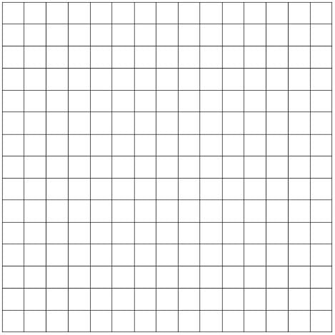
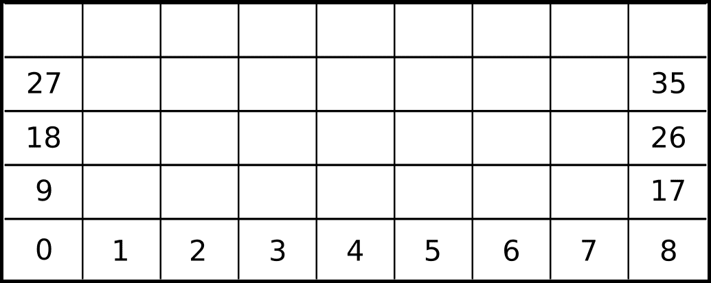
Consider the mesh from the picture below. Its first cells are enumerated, along with the first four left and right boundary cells. This mesh is an example of a rectangular mesh. To illustrate the ease of obtaining cell adjacencies, it’s clear that to obtain the right adjacency from any cell, the problem is reduced to summing one to its enumeration.
Similarly, the top adjacency from any cell is obtained by summing nine to the cell enumeration. This allows for each mesh element to be mapped directly to an array or vector, making computations easier.
Any curvilinear grid can be mapped to such a coordinate and neighboring system. Therefore, from a programming standpoint, there is little to no difference between a curvilinear grid and a rectangular grid in terms of adjacency queries.

Structured grids might also be defined in terms of boundary fitting. For example, a cartesian grid fits the boundary of a rectangle, and a cylindrical grid fits the boundary of a cylinder.
It’s possible to mix the boundary fitting and have many different curves or surfaces that define the boundary. These include any kind of parameterizable curves and surfaces, such as splines and NURBS (Non-Uniform Rational Basis Spline). The meshing algorithm will decide how points will be distributed through those surfaces and how opposing surfaces will be connected to each other, given how many points should be created for each curve or surface.
Unstructured Meshes
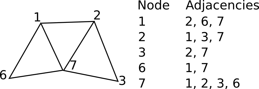
Unstructured meshes are more general and can arbitrarily approximate any geometry shape. In contrast with structured meshes, where the coordinates and connectivities map into the elements of a matrix, unstructured meshes require special data structures, such as an adjacency matrix or list and the node coordinates list. The unstructured mesh node/cell numbering can be arbitrary and sparse since it does not require any analytical form of adjacency query.
Complex geometries that would be impractical to generate a structured mesh within, can be discretized using unstructured meshing techniques. The flexible nature of unstructured meshes allows various cell types to be used and coexist in the same mesh, making it possible to have an even better geometry fitting and overall element quality.
Cell types can be separated into 2-Dimensional cells and 3-Dimensional cells. Common 2-Dimensional cell types are the triangle and the quadrangle. Common 3-Dimensional cell types are the tetrahedron and the hexahedron but might also include the pyramid and wedge.
These cell types form what is sometimes called the finite element zoo since these cell types are commonly used with Finite Element schemes. Finite Volume schemes are known for being more flexible in terms of the cell types being used, sometimes allowing for any kind of polygons and polyhedra.

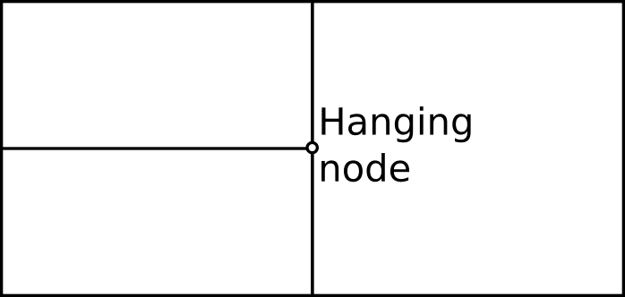
Mesh cells are not required to be conformal. Nonconforming meshes are those where hanging nodes occur. These nodes appear more commonly during mesh adaptation processes.
Generate your own mesh!
Generating a good mesh is the key to an accurate and successful simulation. But hey, it doesn’t have to be perfect the first time you try it. SimScale’s meshing tutorials will help you with all the necessary steps. Become a SimScale member today!
Mesh Adaption
Since on unstructured meshes the points and adjacencies do not follow any kind of global structure, it is also possible to add or remove mesh cells and points. The process of dynamically adding, removing or displacing mesh cells and points is called mesh adaptation.
Depending on the problem nature, mesh adaptation techniques are required to obtain accurate solution fields while maintaining the computational cost low by keeping the overall number of mesh cells and nodes under control. In general, the degree of refinement required is associated with the error, which is estimated based on the equations to be solved. Therefore, regions with higher error will end up accumulating more mesh cells.
Mesh refinement is divided into several general types. Most commonly, these types are referred to as:
- h-type refinement
- r-type refinement
- p-type refinement
- derefinement
- combinations of the above
Mesh Refinement and Derefinement (h-type)
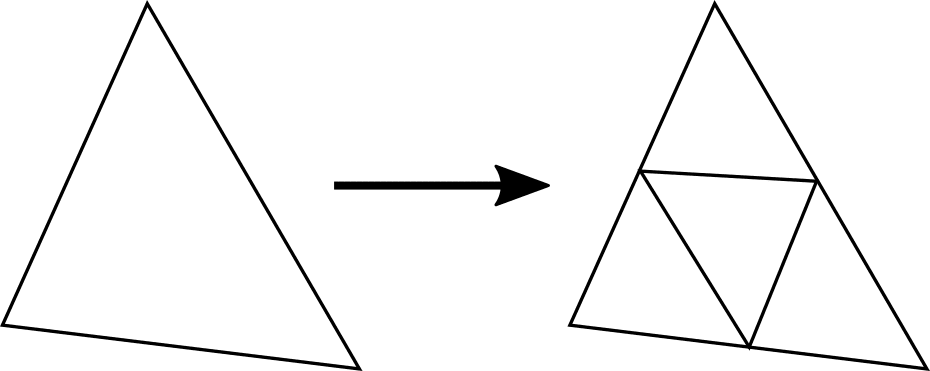
Mesh refinement, which is also called h-type refinement, is based on the addition of cells or points, reducing the local characteristic length of edges. This technique can cheaply increase local mesh resolution but will also increase the number of simultaneous difference equations to be solved since it increases the number of degrees of freedom of the system.
On unstructured meshes, the addition of cells or points is straightforward, as it involves the reconnection of the modified cells. Refinement on structured grids isn’t straightforward since the addition of cells could break the mesh regularity. It’s common to allow for nonconforming meshes when using adaptive structured grids.
Similarly, mesh refinement techniques, in general, allow for mesh derefinement, which can be used to decrease the number of cells in regions where the estimated error is very low. This allows for computational power to be more efficiently used, reducing costs and simulation time.
Mesh Movement (r-type)
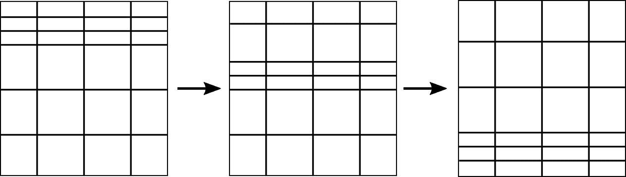
Mesh movement, or r-type refinement, is done through the movement or displacement of mesh cells and points. In this case, the number of cells and points remains constant while also sometimes keeping the connectivity the same.
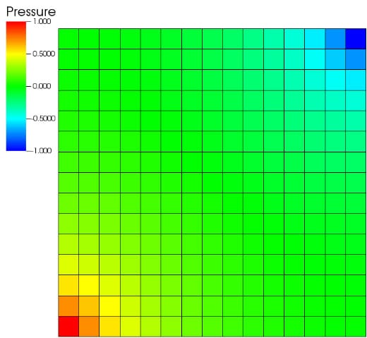
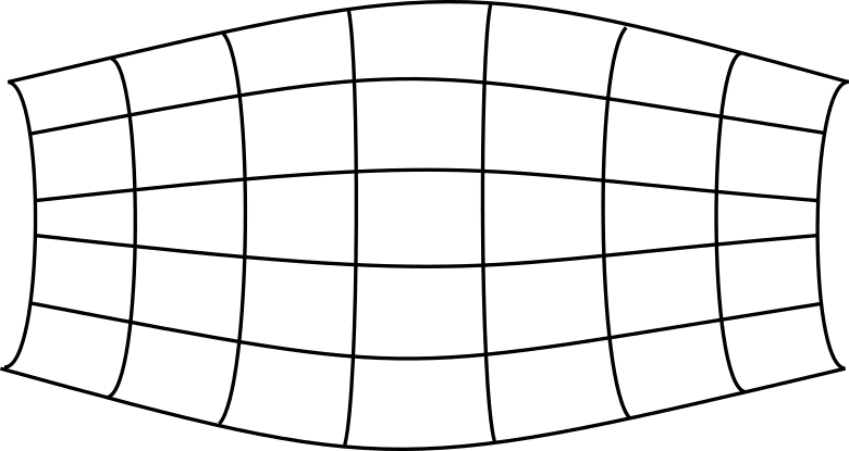
Figure 11 shows an example of an r-type mesh refinement process that could be related to a shock wave propagation problem, for example, where the mesh resolution is kept higher in regions of high variation on the solution.
Other Mesh Adaption Techniques
Other common mesh adaptation techniques might include p-type refinement and adaptive remeshing. On p-type refinement, which is associated with the Finite Element Method, the complexity of the shape function is increased while keeping the same mesh.
The adaptive remeshing technique is used to generate a new mesh based on the estimated error. This allows for the best overall mesh quality and fewer points to be used. On the other hand, the overhead of mesh creation might be large. Adaptive remeshing can be used locally, generating new meshes only in regions where the estimated error is too high or low.
Combinations of the aforementioned techniques can be used. For example, the combination of r-type and h-type refinement can be referred to as rh-type refinement, where nodes can both be displaced or created on the mesh.
Meshing in SimScale
SimScale provides a rich set of meshing algorithms and mesh types, together with comprehensive tutorials.
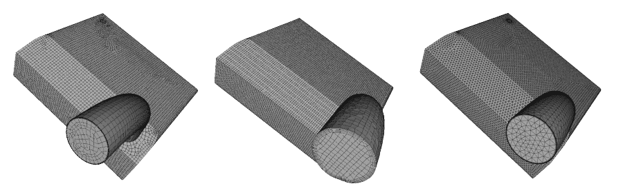
One of the most common examples found on the platform comprises the meshing of a pipe for internal flow simulation. In this example, the process of generating a tetrahedron-dominant mesh is detailed step by step.
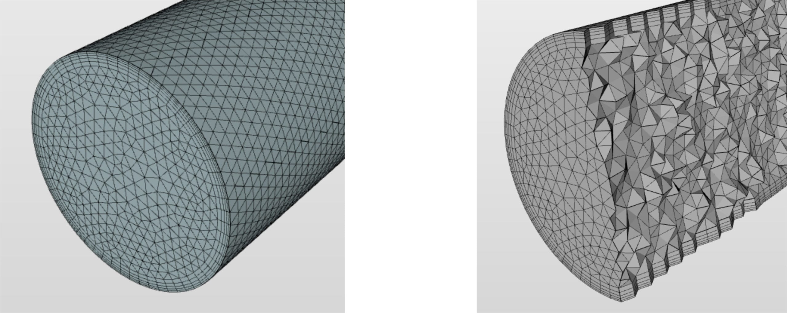
Of the many amazing features, SimScale incorporates the snappyHexMesh feature for its hex-dominant meshing algorithm. It generates 3D- unstructured or hybrid meshes made of hexahedra (hex) and split-hexahedra (split-hex) elements.

References
- Courant, R., Friedrichs, K.O., Lewy, H., “Über die partiellen Differenzengleichungen der Mathematischen Physik”, 1928
- Thomée, V., “From finite differences to finite elements: A short history of numerical analysis of partial differential equations”, 2001
- Thompson, J. F., Soni, B. K., Wheatherill, N. P., “Handbook of Grid Generation”, 1999
Last updated: February 17th, 2023
Did this article solve your issue?
How can we do better?
We appreciate and value your feedback.
What's Next
Background for Hex-dominant

