Numerics

Under Numerics you can set the equation solver for your simulation, change the convergence settings, select algorithms and residuals or choose the time integration scheme for transient dynamic simulations. These settings mainly influence the stability and efficiency of your simulation run, but also the quality of the results may depend on these settings.

All numerical settings are made available for users to have full control over the simulation. These settings can be found for Fluid Dynamics (OpenFOAM®), Multi-purpose, Solid Mechanics (Code_Aster) and Nonlinear Mechanical (MARC) analysis types. The available settings differ based on individual analysis type physics.

Numerics for CFD

In OpenFOAM based analysis types in SimScale the settings for the Numerics section can be categorized into the following:

• Properties

All properties regarding the iterative solvers of velocity and pressure equations are set here. Relaxation factors, non-orthogonal correctors, residual controls, and solver-specific tweaks are among these settings. However, depending on the solver (e.g. PIMPLE, PISO, …), these settings will be adjusted.

• Solver

In this part, linear solvers used in computing each variable could be chosen separately. Upon choosing a solver, a set of preconditioners/smoothers and their tolerances become available. To assist with selecting the best solver, a Help message is provided for each field.

• Numerical Schemes

These schemes determine how each term in the governing equations should be discretized. These are required to evaluate, for e.g., gradient and interpolations of variable terms from cell centers to nodes. In most cases, the standard settings should be a good choice and should not be changed without reason.

Numerics for Radiation

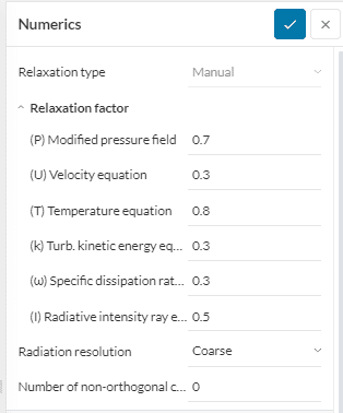
For radiative heat transfer problems, further settings can be changed within the numerics, as shown in the picture below. Most importantly, the radiation resolution can be changed. This affects the discretization of the directions for which the radiative problem is solved. The settings are coarse, moderate, and fine. Increasing the radiation resolution will lead to a higher number of directions and hence improved angular discretization of the radiative problem (usually a more accurate result).

Numerics for Joule Heating

For simulations involving Joule heating, additional settings are available within the numerics, as shown in the picture below. The voltage relaxation factor can be modified to improve the stability and convergence of the numerical solution when solving the voltage equation. Additionally, for the initial iterations of the voltage field, the maximum initial voltage and convergence criteria can be specified. Along with this, the numerics of the voltage solver can also be configured allowing for precise control over the solution process.

Numerics for FEA

Similar to fluid simulations, structural simulations involve linear and non-linear equations that need to be solved. SimScale provides the Numerics settings panel where a user can select algorithms, type of residuals and threshold values, maximum number of iterations, time integration schemes, etc.

A full explanation of the parameters available under these settings can be found here

Structural Analysis Numerics

Numerics for Marc

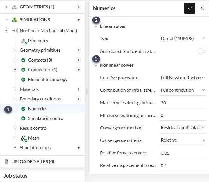
For the Nonlinear Mechanical (Marc) analysis type, the Numerics panel controls the linear and nonlinear solver behavior used to resolve each load increment.

Setting	Options	Description
Type	Direct (MUMPS), Direct (Pardiso), Iterative	The algorithm used to solve the linear system inside every Newton iteration. Direct solvers are memory-intensive but robust for strong nonlinearity and contact.
Auto constrain to eliminate rigid body motions	On, Off	Only relevant when a direct solver is used. Adds small artificial stiffness to prevent singularities from unconstrained bodies before contact engages.

Nonlinear Solver

Setting	Options	Description
Iterative procedure	Full Newton-Raphson, Modified Newton-Raphson, Newton-Raphson with strain correction	Full Newton-Raphson recomputes and refactorizes the stiffness matrix at every iteration, giving the fastest convergence at a higher per-iteration cost — the standard choice for strongly nonlinear problems such as large deformation, contact, and nonlinear materials.
Contribution of initial stress to stiffness	Full contribution, no contribution, only positive stress, hydrostatic-pressure-reduced, stress at start of increment, only positive principal stresses	Determines how much of the geometric (stress) stiffness is included in the stiffness matrix. Full contribution is standard for large-displacement or buckling-sensitive analyses.
Max recycles during an increment	Integer	The maximum number of equilibrium iterations allowed within one time increment before the increment is cut back or the analysis is halted.
Min recycles during an increment	Integer	The minimum number of iterations forced per increment, guarding against false early convergence.
Convergence method	Residuals, Displacement, Strain energy, Residuals or displacements	Determines whether equilibrium is judged by force residuals, displacement, strain energy, or a combination.
Convergence criteria	Relative, Absolute	Whether the convergence tolerances are expressed relative to the reaction forces or as absolute values.
Relative force tolerance	Fraction, e.g. 0.05	When Convergence criteria is Relative, convergence is declared once the ratio of maximum residual force to maximum reaction force drops below this value.
Auto switch method	On, Off	Lets Marc automatically switch the convergence testing method if the residual-based check becomes numerically unreliable, for example near-zero reactions.

Last updated: September 24th, 2026