Tutorial: Frequency Analysis of an Airfoil (1/2)

This is a tutorial about how to set up a frequency analysis of an airfoil and how to visualize the results. Note that this is the first tutorial of a series: In this tutorial, we are analyzing the eigenfrequencies which are the basis for the harmonic analysis done in the second tutorial, Harmonic Analysis of an Airfoil.

This tutorial teaches how to:

• Set up and run a frequency analysis.
• Assign boundary conditions, material and other properties to the simulation.
• Mesh with the SimScale standard meshing algorithm.

You will be following the typical SimScale workflow:

1. Preparing the CAD model for the simulation.
2. Setting up the simulation.
3. Creating the mesh.
4. Run the simulation and analyze the results.

1. Prepare the CAD Model and Select the Analysis Type

First of all click the button below. It will copy the tutorial project containing the geometry into your own workbench.

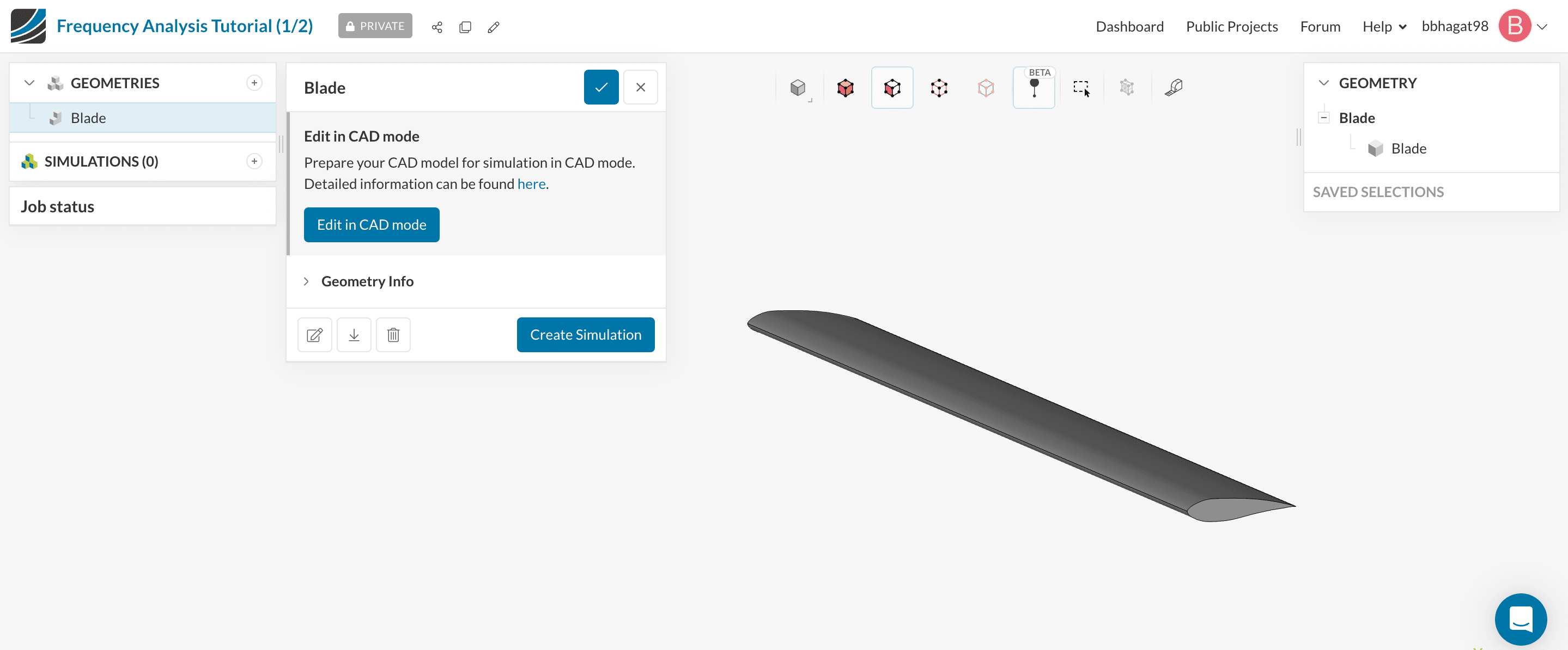
The following picture demonstrates what should be visible after importing the tutorial project.

1.1. Create the Frequency Analysis Simulation

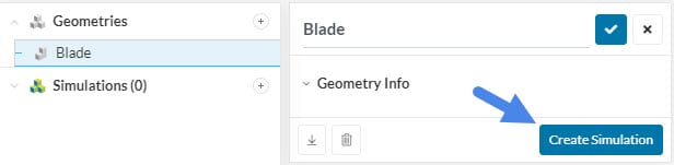
Once the geometry is in the platform, click on it, and then choose the ‘Create Simulation’ option:

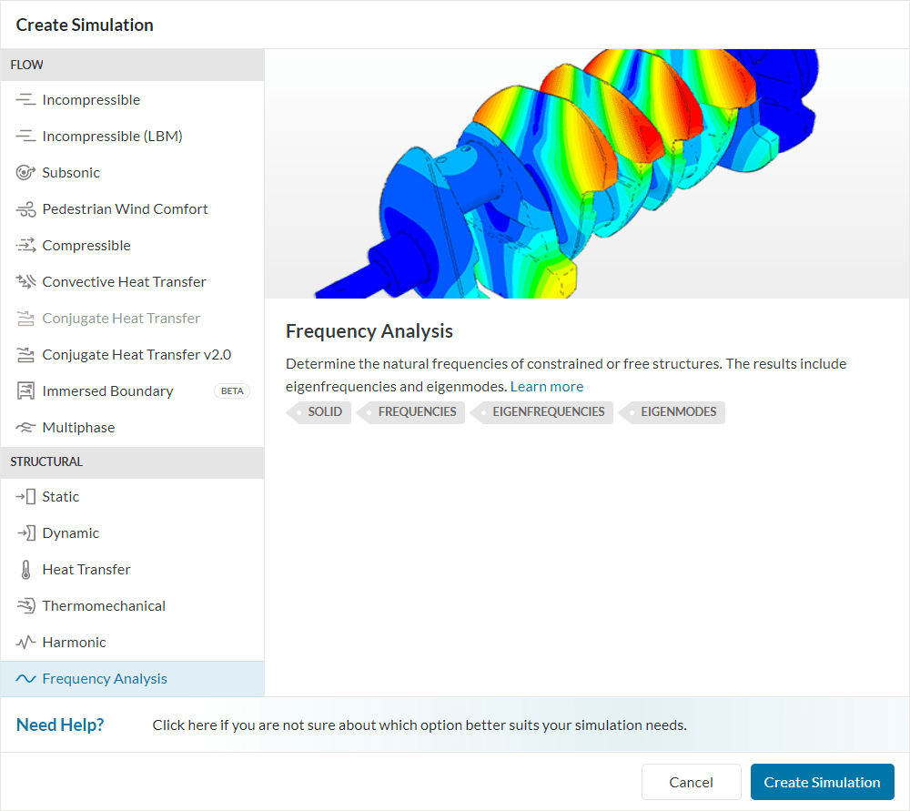
Then select the ‘Frequency Analysis’ type.

2. Set Up the Simulation

2.1. Materials

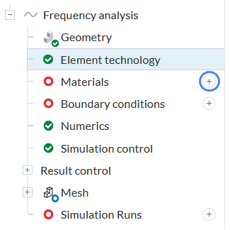
The SimScale platform comes with a large number of default materials. In order to add a new one, click on the ‘+’ next to the Materials tab.

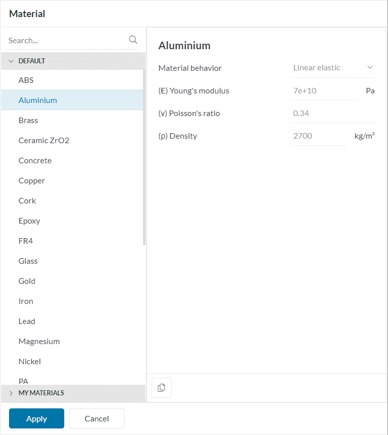
A solid material is fitting for this kind of frequency analysis. Select the ‘Aluminium‘ from the Material list that will appear and hit ‘Apply’.

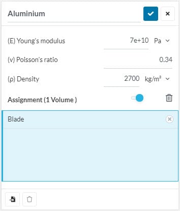
The blade will be assigned automatically. Leave the material properties at their default state.

2.2. Boundary Conditions for the Frequency Analysis

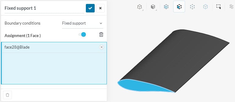
Apply fixed support to the side face of the airfoil. Start by clicking on the ‘+’ icon next to the Boundary Conditions, and then picking the ‘Fixed Support’ option from the menu. This way, the assigned face will be fully constrained.

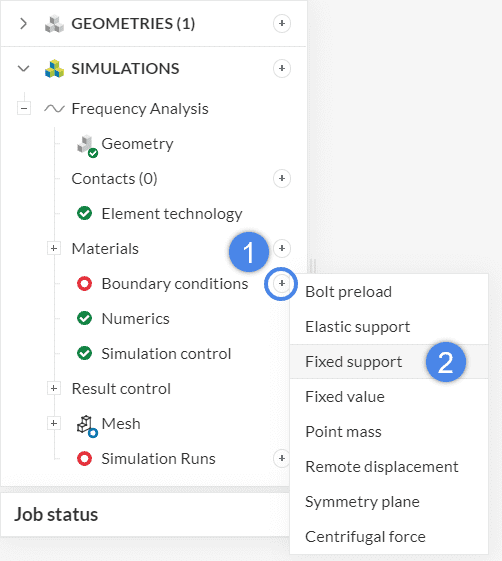
Apply a fixed support to the side face of the airfoil.

2.3. Simulation Control & Frequency Analysis Numerics

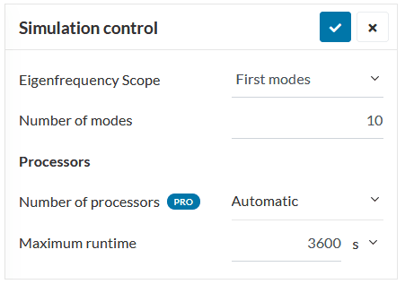
The default values for the Numerics are fine for this simulation.
Within simulation control, the eigenfrequency scope must be set to first modes, with the number of modes being equal to \(10\), as its default value.

3. Mesh

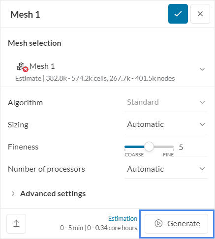
The standard mesher will be used. For this tutorial, keep all settings as default and hit ‘Generate’. For linear FEA simulations, SimScale will create a 2nd order mesh by default, which aims for more precision in FEA studies (definition under the Element technology tab).

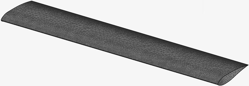
The resulting mesh will look like this:

4. Start the Simulation

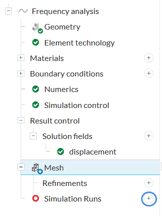
In order to create a new run, click on the ‘+’ next to the Simulation Runs:

Now you can start the simulation. While the results are being calculated you can already have a look at the intermediate results in the post-processor. They are being updated in real-time!

5. Post-Processing

After about 18 minutes you can have a look at the results.

5.1 Eigenmodes & Eigenfrequencies

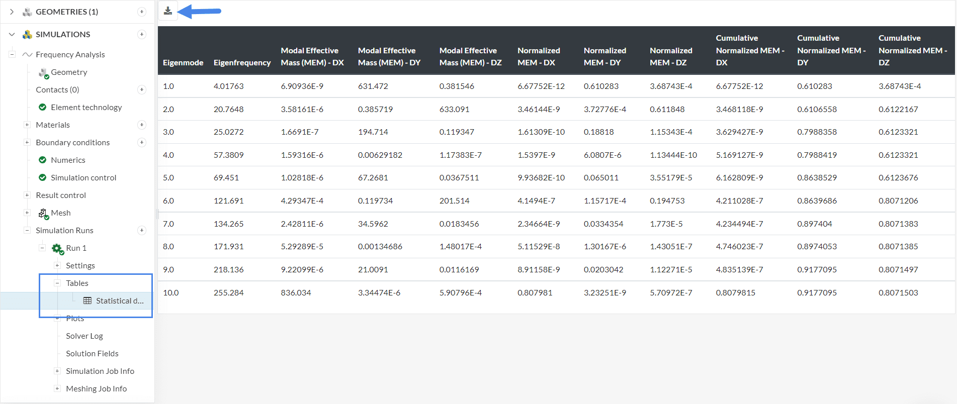
When expanding the information of the finished run, there is a Statistical Data section under the Plots, that includes the calculated eigenfrequencies. You can view the data, or even download them by clicking on the icon at the top of the table as highlighted below:

5.2 Surface Visualization

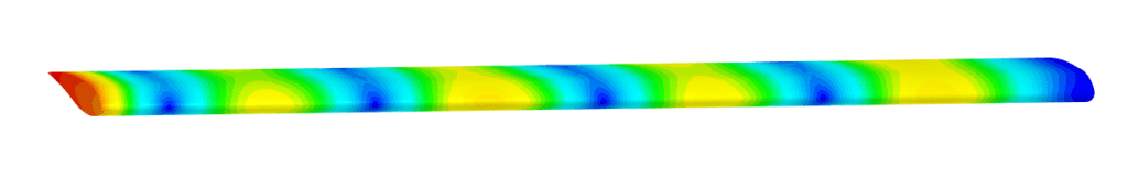
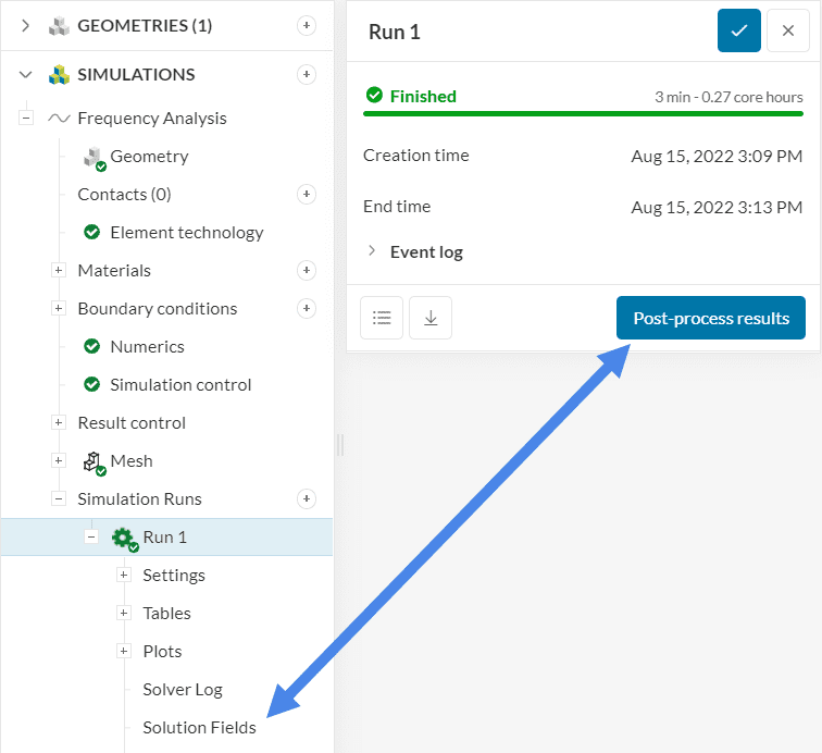
In order to view the results of your frequency analysis, click on the ‘Post-process results‘ tab under your finished run.

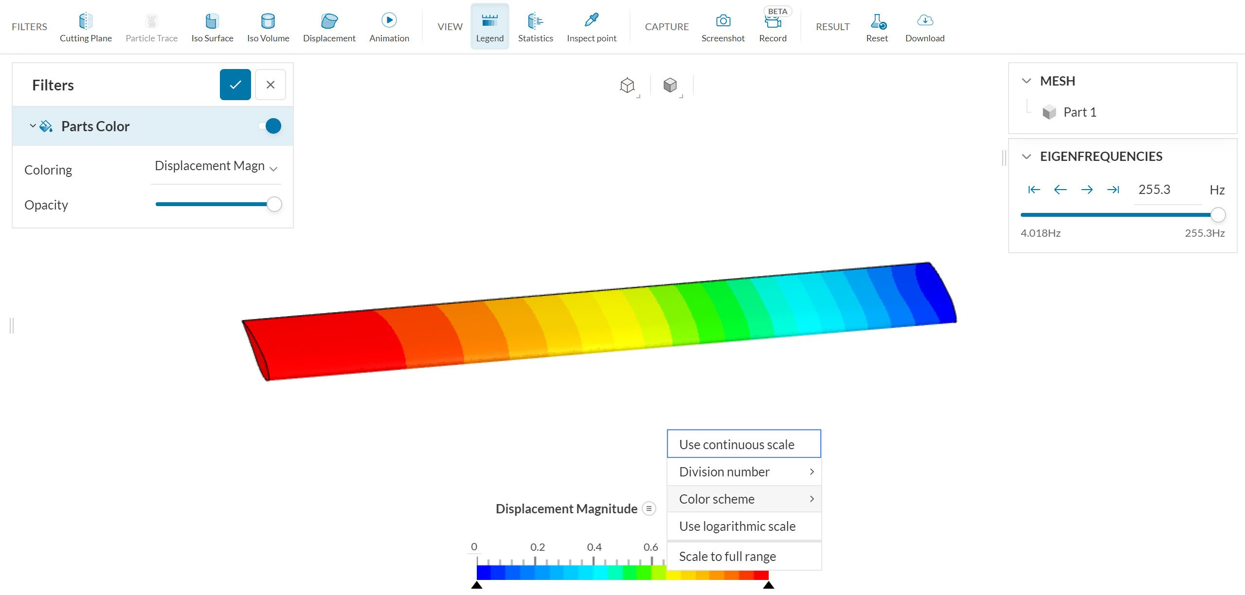
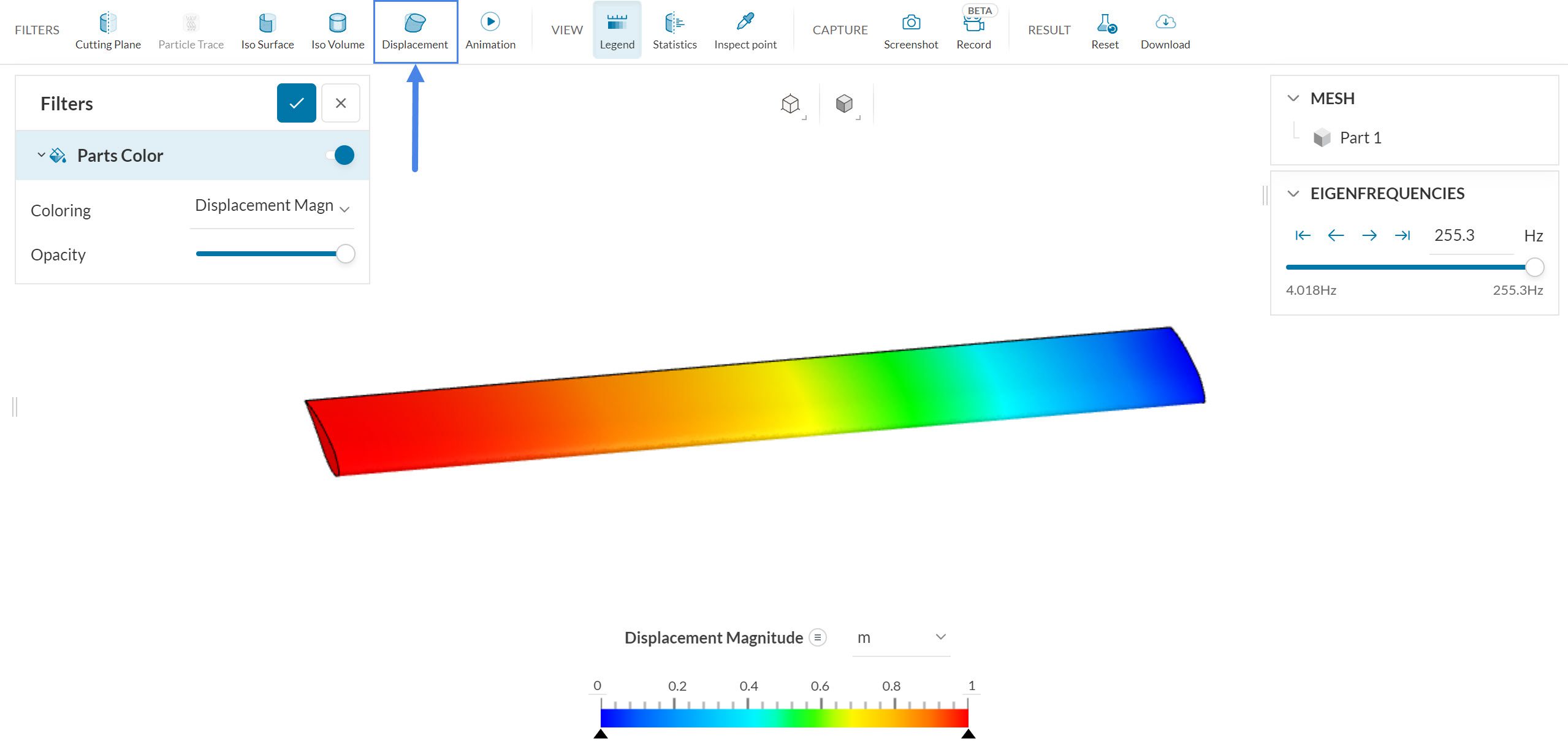
Choose the “Displacement Magnitude” to display on your part as Coloring. In order to improve the quality of your visualization, and make the color transition smoother, right-click on the legend bar at the bottom, and select the ‘Use continuous scale‘ option:

You can visualize more parameters by changing the Coloring input.

5.3 Displacement

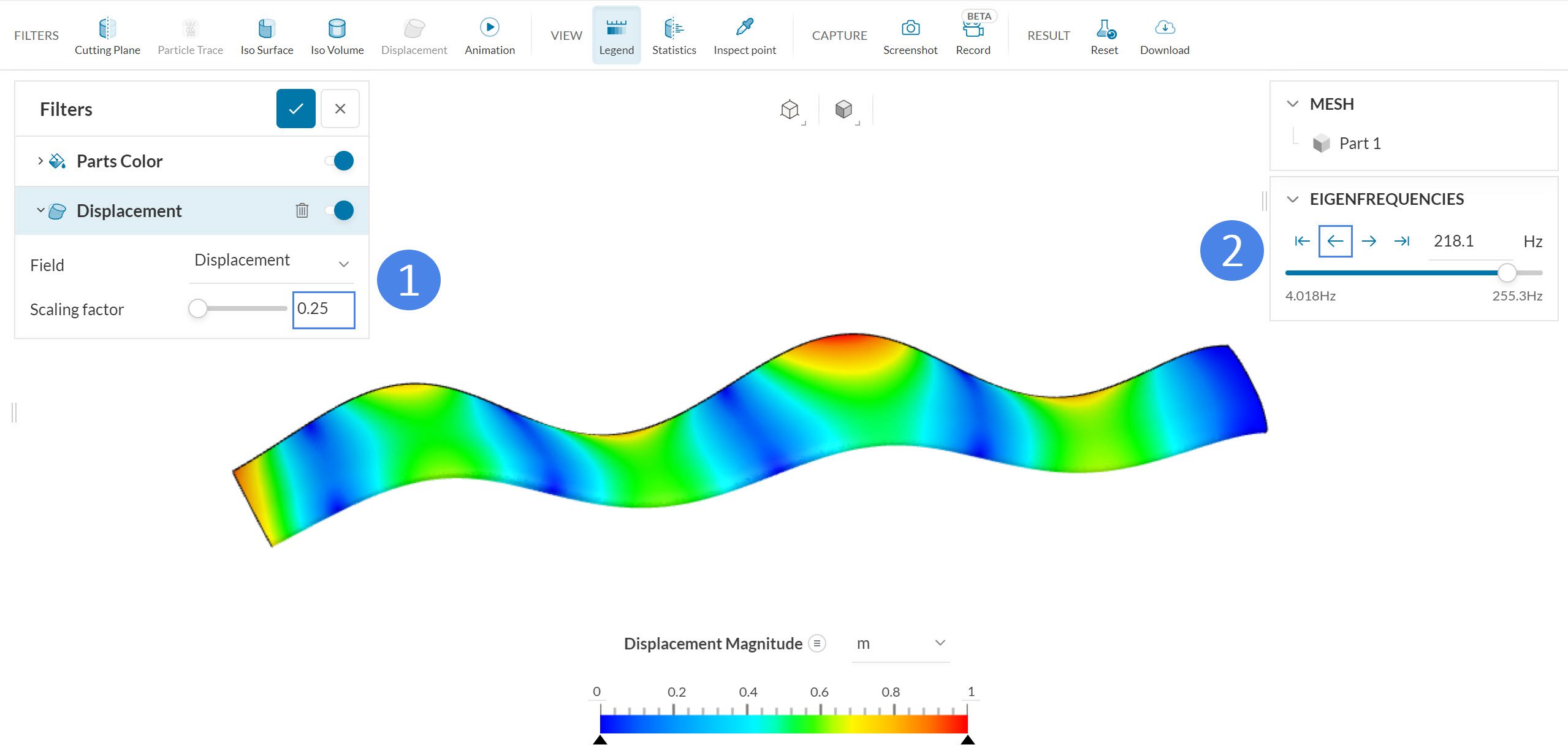
There are more features to use in order to post-process the results of the run, and you can access them by clicking on the ‘Add filter’ option. Then the menu with all the available options appears:

Select ‘Displacement‘ from the menu. You will notice that there is no difference after you create this new filter, so apply the following settings:

• Set the Scaling factor to ‘0.25’. This will only change the physical deformation of the model, and for this simulation, the scale was brought down to 0.25 because it makes the natural frequencies easier to identify.
• Rollback to the previous written timestep, which represents the 9th eigenfrequency shown in Figure 14. Each step is a different frequency, and you can display whichever you wish.

With a frequency analysis, one can determine the natural frequencies for a geometry. This information is valuable and can be used to get more meaningful results in the harmonic analysis that comes in the next step. Make sure to check the Harmonic Analysis of an Airfoil to learn more!

Analyze your results with the SimScale post-processor. Have a look at our post-processing guide to learn how to use the post-processor.

Congratulations! You finished the tutorial!

Last updated: November 29th, 2023