Tutorial: Harmonic Analysis of an Airfoil (2/2)

This article provides a step-by-step tutorial for a harmonic analysis simulation of an airfoil, including post-processing. It is a continuation of the Frequency Analysis of an Airfoil (1/2) tutorial.

This tutorial teaches how to:

• Set up and run a harmonic simulation;
• Assign boundary conditions, material, and other properties to the simulation;
• Mesh with the SimScale standard meshing algorithm.

We are following the typical SimScale workflow:

1. Prepare the CAD model for the simulation;
2. Set up the simulation;
3. Create the mesh;
4. Run the simulation and analyze the results.

1. Prepare the CAD Model and Select the Analysis Type

In case you already have a project from the Frequency Analysis of an Airfoil Tutorial, feel free to continue using that Workbench. The geometry and mesh are the same as in the frequency analysis tutorial.

Otherwise, you can click the button below. It will copy the tutorial project containing the geometry into your Workbench.

The following picture demonstrates what should be visible after importing the tutorial project.

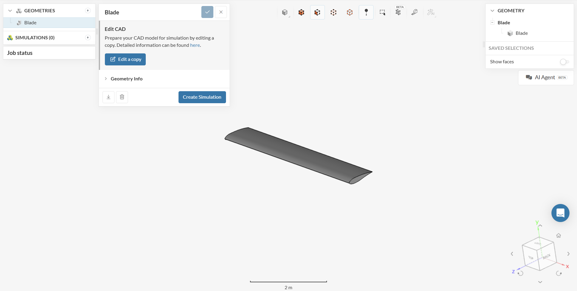
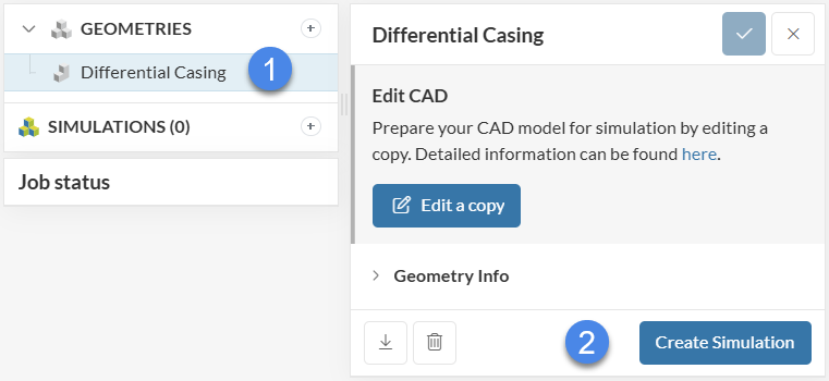
1.1 Create the Simulation

As a first step, click on the geometry name.

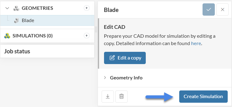
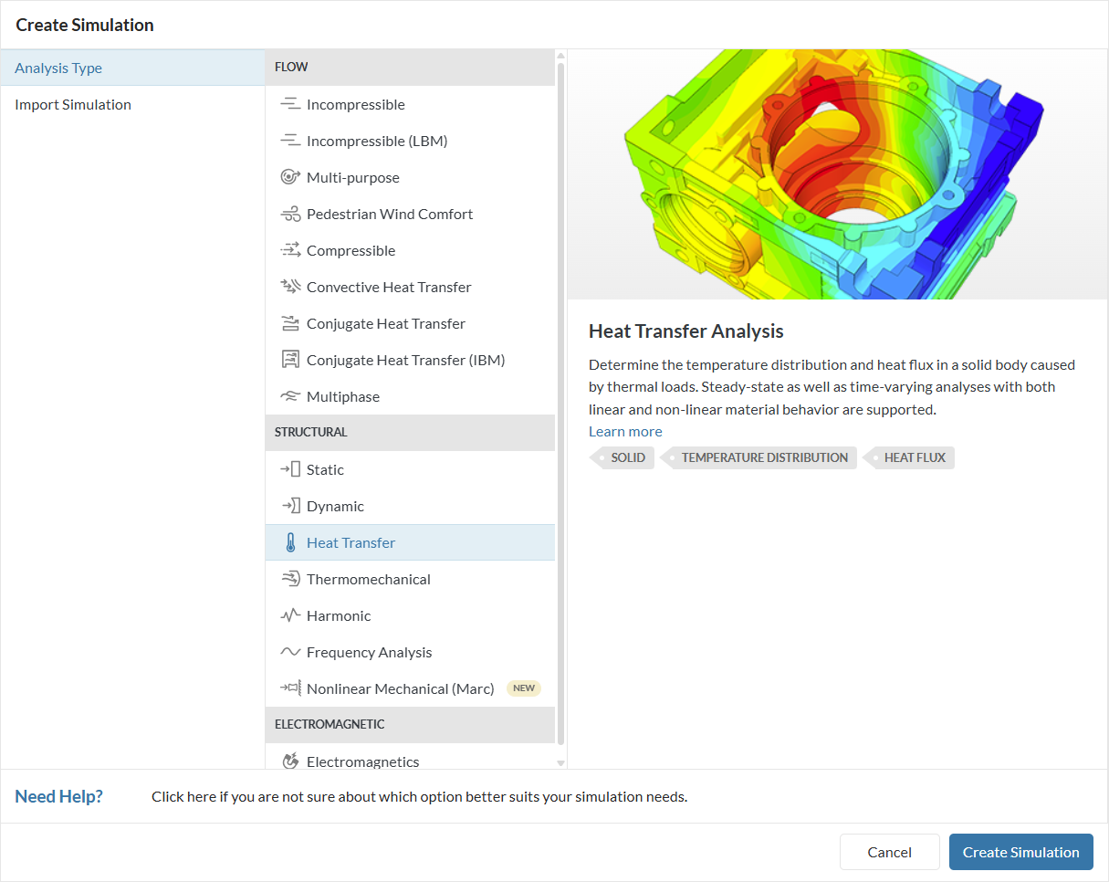
Hitting the ‘Create Simulation’ button leads to the following options:

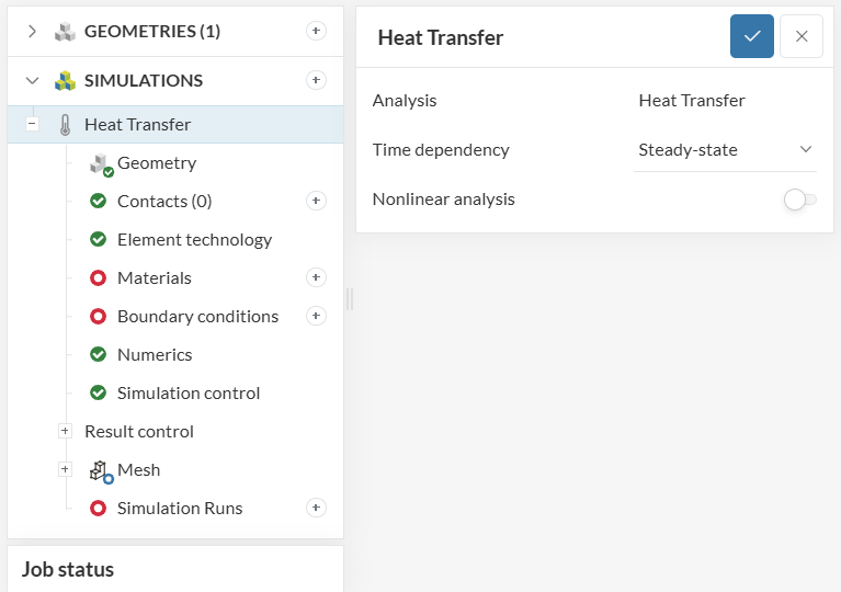
Choose ‘Harmonic‘ as the analysis type and ‘Create the Simulation‘.

2. Assigning the Material and Boundary Conditions

The following picture shows an overview of the boundary conditions applied for this simulation:

We will assign a pressure load at different eigenfrequencies based on the results of the frequency analysis tutorial as well as fixed support. Furthermore, we are going to use aluminum as a material for the wing.

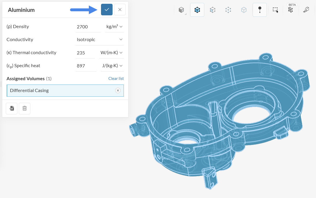
2.1 Define a Material

In the left-hand side panel, click on the ‘+ button‘ next to the Materials. In doing so, a list of pre-defined material appears.

Choose ‘Aluminium‘ from the library and hit ‘Apply‘.

Now you successfully created the material. The blade is assigned to it automatically. All you need to do is confirm it by hitting the checkbox next to Aluminium.

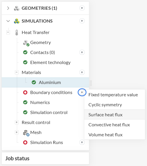
2.2 Assign the Boundary Conditions

In the next step, boundary conditions need to be assigned, using Figure 4 as a reference. For an overview of the boundary conditions available, please have a look at this documentation page.

a. Fixed Support

The first boundary condition is fixed support. It represents zero displacement in all directions. Proceed as below:

After hitting the ‘+ button’ next to boundary conditions, a drop-down menu opens. From it, one can choose between different boundary conditions. After choosing ‘Fixed support‘, assign it to one of the airfoil’s tips:

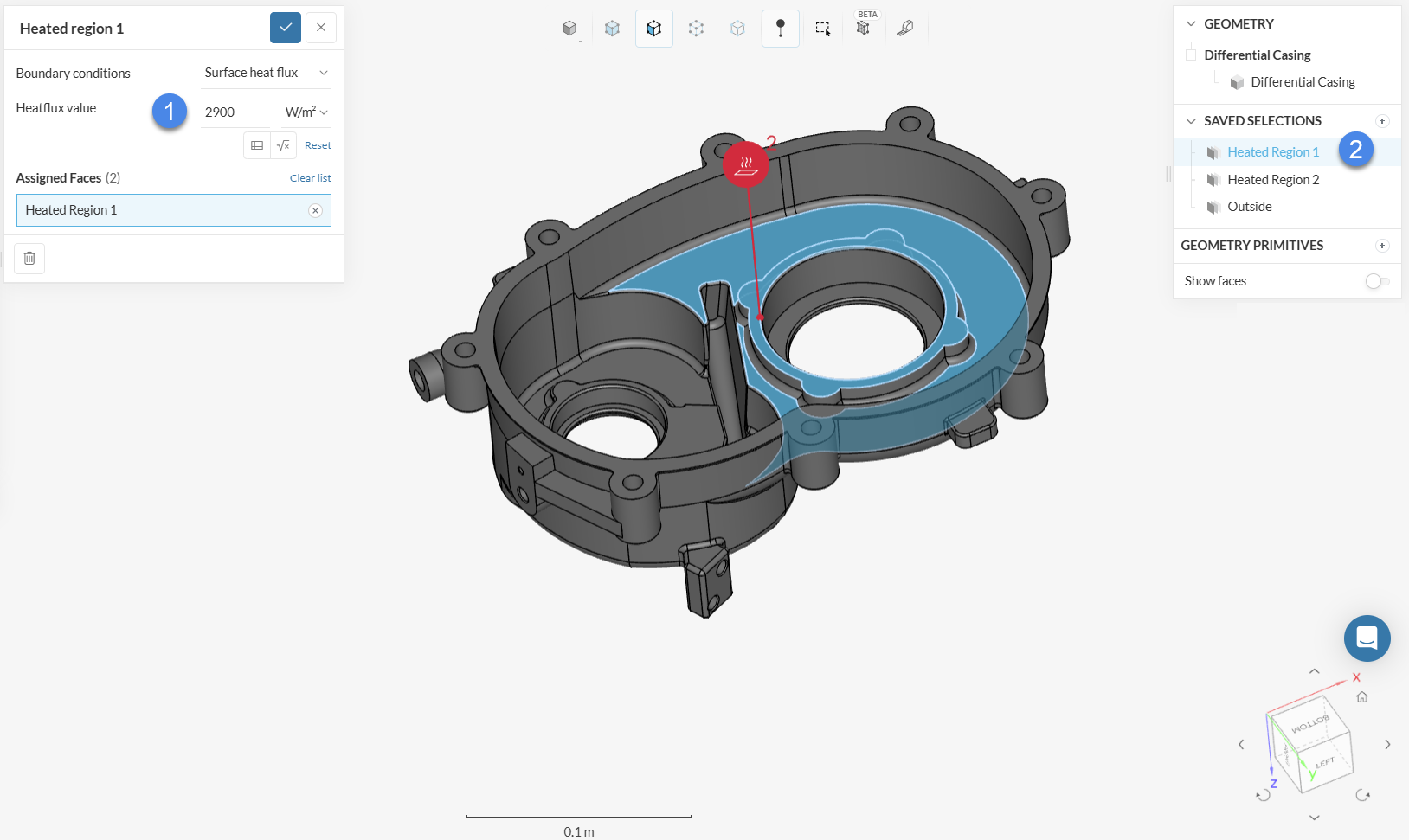
b. Pressure

Still based on figure 4, create a second boundary condition and choose ‘Pressure‘. This will be used for the harmonic excitation. Let’s apply a pressure of ‘500‘ \(Pa\) on the bottom face of the airfoil. Phase angle should be kept at 0 degrees in case of a single force.

For applications where more than one force is applied, oftentimes a non-zero phase angle will be specified. For example, in a car engine analysis, we have several pistons with unsynchronized forces. In this case, you can set one of the forces with a phase angle of 0 and define the phase of the other forces accordingly.

2.3 Numerics and Simulation Control

Under Simulation control, you can specify a list of Excitation frequencies, at which the loads will be excited. To specify meaningful excitations for the harmonic analysis, it is important to perform a frequency analysis on the geometry, to gain more insight into the natural frequencies.

Therefore, the results from the frequency analysis tutorial are important in this step. These are the first 10 modes for the airfoil geometry and their respective natural frequencies. You can find the following figure in the results of the frequency analysis tutorial here:

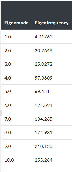
These 10 frequencies span from 4 to 255 \(Hz\). Let’s focus on the first 3 modes for the harmonic analysis.

In Simulation control, change the settings to the following:

• Set Excitation frequencies to ‘Frequency list‘;
• Change Start frequency to ‘2.5‘ \(1/s\);
• End frequency is ‘30‘ \(1/s\);
• Frequency stepping will be ‘2.5‘ \(1/s\). With these settings, a total of 12 frequencies will be analyzed.

2.4 Result Control

With result controls, users can monitor parameters in points of interest within the geometry.

To set up a point control, proceed as below:

1. Click on the ‘+ button‘ next to Point data;
2. Make sure Field selection is set to ‘Displacement‘. Component selection is ‘All‘ and Complex number is ‘Magnitude and phase‘;
3. Lastly, click on the ‘+ button‘ next to Geometry primitives to specify a point.

For the coordinates, specify ‘0.1‘ in the x-direction, ‘0‘ in the y-direction, and ‘-0.8‘ in the z-direction:

After saving the probe point, it is automatically assigned to the probe point result control.

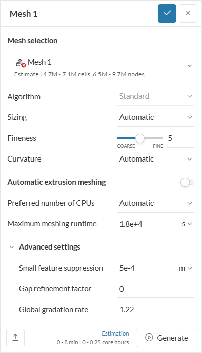
3. Mesh

To get the mesh, we recommend using the Standard algorithm, which is a good choice in general as it is quite automated and delivers good results for most geometries.

This tutorial uses the same mesh from the frequency analysis tutorial. Therefore, please keep all settings as default and hit ‘Generate’. The resulting mesh will be a second order mesh (see the element technology tab), which is optimal for accuracy.

After a few minutes, the mesh is ready and looks like this:

4. Start the Simulation

Now you can start the simulation. While the results are being calculated you can already have a look at the intermediate results in the post-processor. They are being updated in real-time!

5. Post-Processing

After around half an hour, the results should be available.

5.1 Displacement Plots

First, let’s have a look at the result controls that we specified. Recalling the natural frequencies, we can see that peaks in displacement occur around those frequencies:

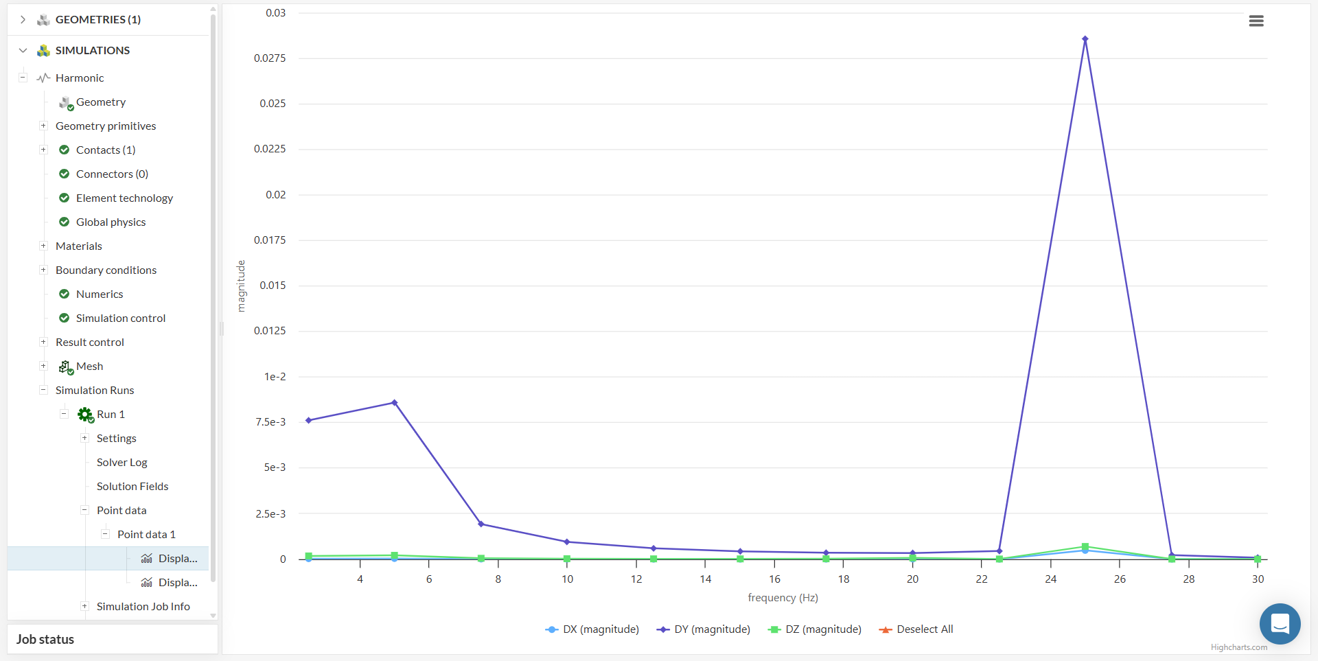
The phase angles observed for this simulation are either 0 or 180 degrees. This indicates that the peaks in both displacement and forces occur at the same time.

5.2 Surface Visualization

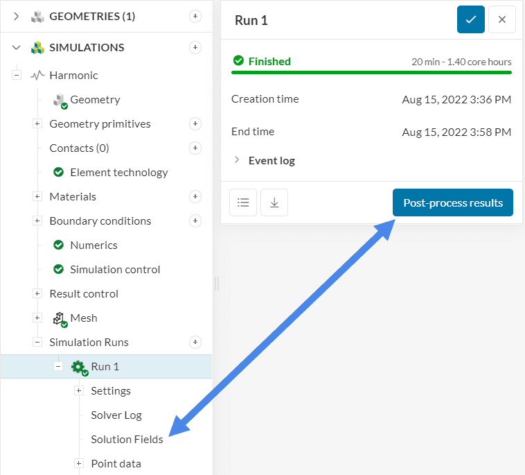
To view the results of your harmonic analysis, click on the ‘Post-process results‘ tab under your finished run.

Make sure that ‘Von Mises Stress (real)’ is displayed on the part, under the Coloring section. To improve the quality of your visualization, and make the color transition between blocks smoother, right-click on the legend bar at the bottom of the page, and select the ‘Use continuous scale’ option:

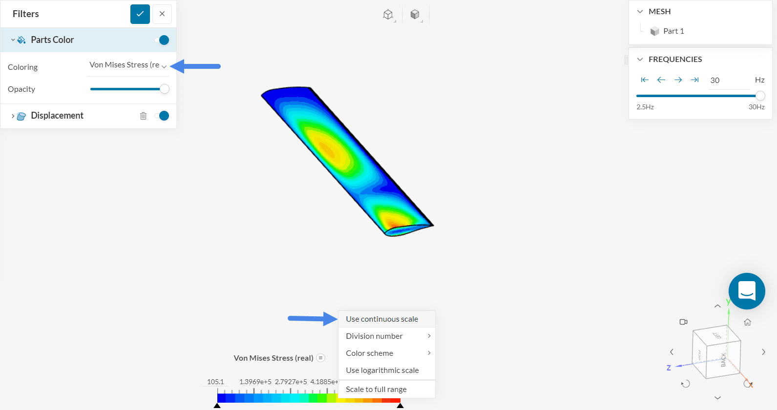
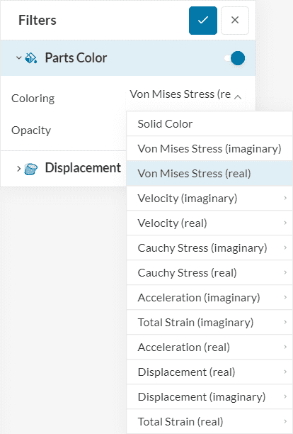
You can visualize more parameters by changing the Coloring input:

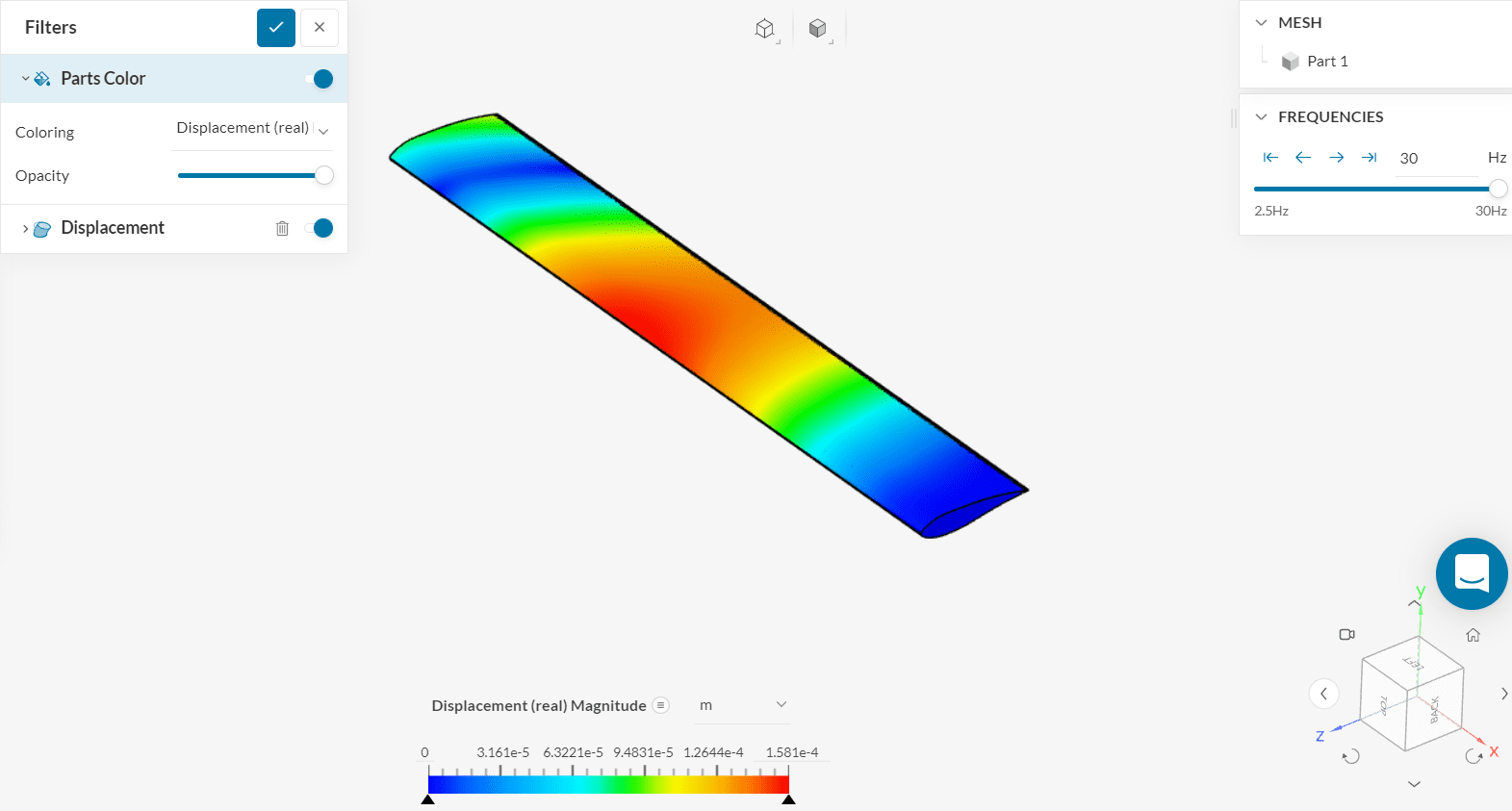
For example, this is what the surface visualization with the real displacement values looks like when the continuous scale feature is also added:

5.3 Displacement

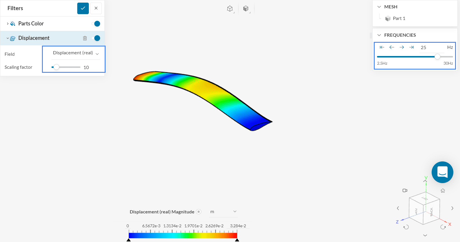
The default state of the post-processor contains the Displacement filter. This filter allows you to visualize (and magnify) the displacements in the viewer.

Plotting displacement contours can also provide valuable insight into the behavior of the parts. Below, we have activated the visualization of displacements. For 25 \(Hz\), a bending effect occurs and the displacement is the largest, as seen in Figure 16. You can check this by implementing the following:

• Change the Fields to ‘Displacement(real)‘;
• Set the Scaling factor to 10, making the displacement easier to identify;
• Rollback to the timestep that corresponds to 25 \(Hz\), using the Frequencies slider. You can check other frequencies as well by changing this input.

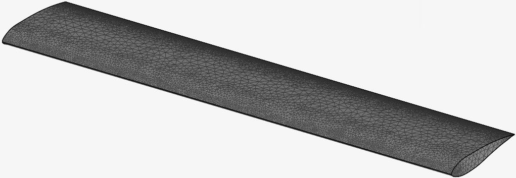
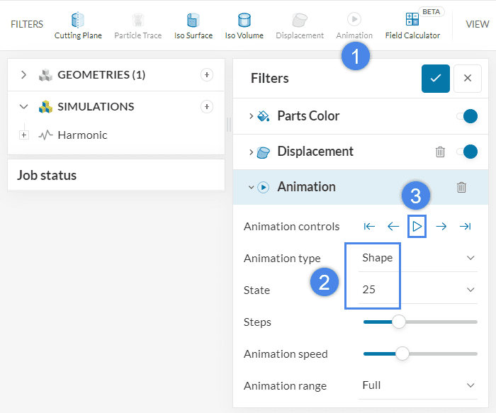
Finally, it’s possible to animate a mode of interest, to see how the structure behaves. By creating an ‘Animation’ filter, and setting the Animation type to ‘Shape’, you will obtain the results shown in the first image of this tutorial.

Analyze your results with the SimScale post-processor. Have a look at our post-processing guide to learn how to use the post-processor.

Congratulations! You finished the tutorial!

Last updated: February 8th, 2023