Documentation
With our Pedestrian Wind Comfort (PWC) analysis, it is possible to input additional advanced modeling of geometry in the form of surface roughness and porous media. This helps to better capture local effects on the wind comfort simulation for a more accurate analysis.
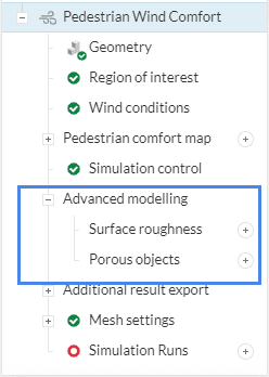
In PWC simulations, wind flow is affected by friction surfaces as well as obstacles, such as terrain, buildings, and trees. As large obstacles are captured via the geometry input, small obstacles or surface roughness is modeled using the advanced surface roughness modeling method. While the effect of surface roughness for laminar flows is negligible, turbulent flows are highly dependent on wall roughness. As the surface roughness changes, the thickness of the viscous sublayer modifies the law-of-wall for mean velocity. As a result, the turbulent friction factor increases with the roughness ratio.
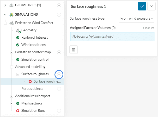
To apply the roughness effects on any surface in PWC analysis, SimScale has three options to input a surface roughness type. To assign a new surface roughness click on the plus icon next to Surface roughness.
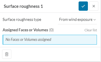
Using the Wind Exposure method the aerodynamic roughness value is automatically selected individually based on the selected wind exposure category for each wind direction. This method is preferred in order to achieve horizontal homogeneity for the incoming ABL flow.
For the exact values of the aerodynamic roughness used, depending on the wind engineering standard, please have a look at this documentation page.
When the roughness of the specific surface is known the Equivalent sand grain method allows the direct assignment of a surface roughness value. Typical values reach from 0.05 \(mm\) for steel to 3 \(mm\) for concrete.

In the following table, the equivalent sand-grain roughness of some materials and terrain types can be seen:
| Material | \(k_{s}\), equivalent sand-grain roughness \([m]\) |
|---|---|
| Concrete, smooth wall | 0.0045 |
| Concrete, rough wall | 0.013 |
| Concrete, floor | 0.04 |
| Rubble | 0.0175 |
| Farmland | 0.135 |
| Farmland with crops | 0.525 |
| Grass with shrubs | 0.265 |
| Shrubbery | 0.5 |
| Grass and stone grid | 0.0225 |
| Gravel | 0.075 |
| Case iron | 0.000254 |
| Commercial or welded steel | 0.00004572 |
| PVC | 0.000001524 |
| Glass | 0.000001524 |
| Wood | 0.0005 |
| Cast iron | 0.00026 |
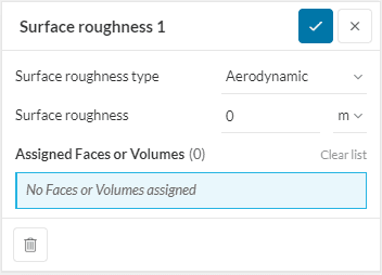
The Aerodynamic surface roughness type is used to model the large-scale effects of non-modeled obstacles on the atmospheric boundary layer flow, such as vegetation, or benches. Typical values range from 0.0002 \(m\) for open sea to 1 \(m\) for dense urban areas. A few example values can be found in Table 2.
| Terrain description | \(z_0\) \([m]\) |
| Open sea, fetch at least 5 \(km\) | 0.0002 |
| Mudflats, snow: no vegetation, no obstacles | 0.005 |
| Open flat terrain: grass, few isolated obstacles | 0.03 |
| Low crops: occasional large obstacles, \(x \over\ H\) > 20 | 0.10 |
| High crops: scattered obstacles, 15 < \(x \over\ H\) < 20 | 0.25 |
| Parkland, bushes: numerous obstacles, \(x \over\ H\) ≈ 10 | 0.5 |
| Regular large obstacle coverage (suburb, forest) | 1.0 |
Where \(x \over\ H\) is the ratio of length to the height of the obstacle.
Porous media is a medium filled with solid particles, which lets fluid pass through. The arrangement of the flow path inside the porous medium can be regular or irregular.
A porous medium can be classified as follows:
Porous media is used to model permeable obstructions such as trees, hedges, windscreens, and other wind mitigation measures. When air flows through a porous body, a pressure gradient along the direction of the flow is generated. Using porous media simplification reduces the CAD and mesh complexity, and saves computational time and expenses.
Within the PWC analysis type, SimScale allows users to model porous objects using the following two models:
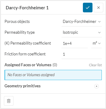
A model used when the pressure drop characteristics of the geometry are known is the ‘Dary-Forchheimer Model’. The model uses a formulation of the pressure drop with respect to the local velocity. The two coefficients used can be determined by a curve fit to experimental data.
The pressure loss due to porosity is modeled by the empirical Darcy-Forchheimer equation.
$$\overline{\frac{\Delta {p}}{\Delta x}}=- \frac{\mu}{K}.\overline{u}-\rho.\frac{F_\varepsilon}{\sqrt{K}}.|\overline{u}|.\overline{u}\tag{1}$$
The first and the second term on the right-hand side of the equation are the Darcy and Forchheimer terms respectively. The Darcy term accounts for the friction drag which has a linear relation to the local velocity vector. The Forchheimer term accounts for the inertial drag or the form drag which has a quadratic relation to the local velocity vector.
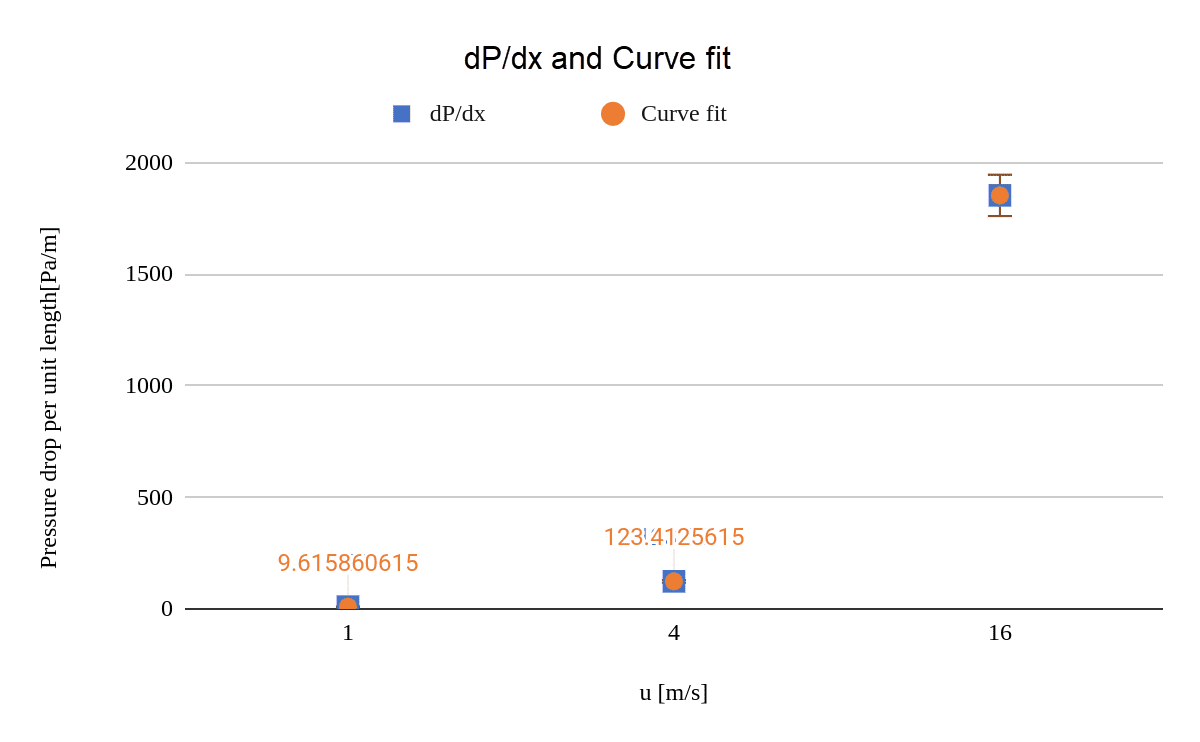
To be able to define a porous media in SimScale, define \(K\) and \(F_\varepsilon\). Use a minimum of 3 data points to perform a curve fitting to predict the \(K\) and \(F_\varepsilon\). An example is shown below:
Experimental data:
| u \([m/s]\) | dP/dx \([Pa/m]\) |
|---|---|
| 1 | 9.88 |
| 4 | 123.33 |
| 16 | 1852.84 |
Curve equation for air:
$$ \frac{\mathrm dP}{\mathrm d x} = \frac{0.0000181}{K}.u+1.\frac{F_\varepsilon}{K^{0.5}}.u^2 \tag{2} $$
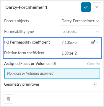
Using the curve-fitting method, the missing coefficients were calculated as follows:
Once the relevant coefficients are calculated, they can be assigned to Darcy-Forchheimer’s porous object definition, and the porous media geometry is selected. This selection can be in the form of faces, volumes, or geometry primitives.
While the isotropic type adds specific resistance in every direction, directional resistance can be added where the specific resistance can be defined for each direction individually.
Tree models are used to model the vegetation (single trees, bushes, hedges, forest canopies, etc.) as porous mediums. It’s possible to either define the porosity as predefined for the five most common trees in EU cities or by creating a custom tree model.
Creating a custom tree requires the following inputs:
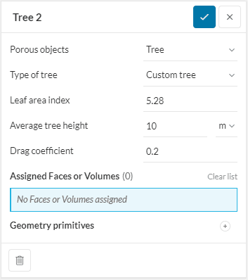
The leaf area index (LAI) is a dimensionless number, which is used to compare plant canopies. It can be simply defined as the total leaf area per unit ground area.
For predefined tree models, only the assignment of tree height is required since the solver applies related LAI and drag coefficient automatically. In SimScale the following models are available.
The following table displays the default trees, and their respective LAI along with the drag coefficient:
| Tree Type | Drag Coefficient | Leaf Area Index (LAI) |
|---|---|---|
| Plane tree | 0.2 | 5.28 |
| Oaktree | 0.2 | 5.1657 |
| Sycamore | 0.2 | 2.9675 |
| Silver birch | 0.2 | 3.2379 |
| Chestnut | 0.2 | 5.1972 |
The above information obtained\(^2\) is a compiled data ranging over 70 years from 500 different locations.
In the tree model, we used the modified Darcy-Forchheimer equation. By assigning a high permeability value, we neglected the Darcy portion and simplified the equation as follows:
$$\frac{\Delta \overline{p}}{\Delta x}=-\rho.\frac{F_\varepsilon}{\sqrt{K}}.|\overline{u}|.\overline{u}\tag{3}$$
Next, modified the equation to define it with respect to Drag Coefficient \(C_d\) and Leaf Area Density \(LAD\):
$$\frac{\Delta \overline{p}}{\Delta x}=-\rho.LAD.C_d.|\overline{u}|.\overline{u}\tag{4}$$
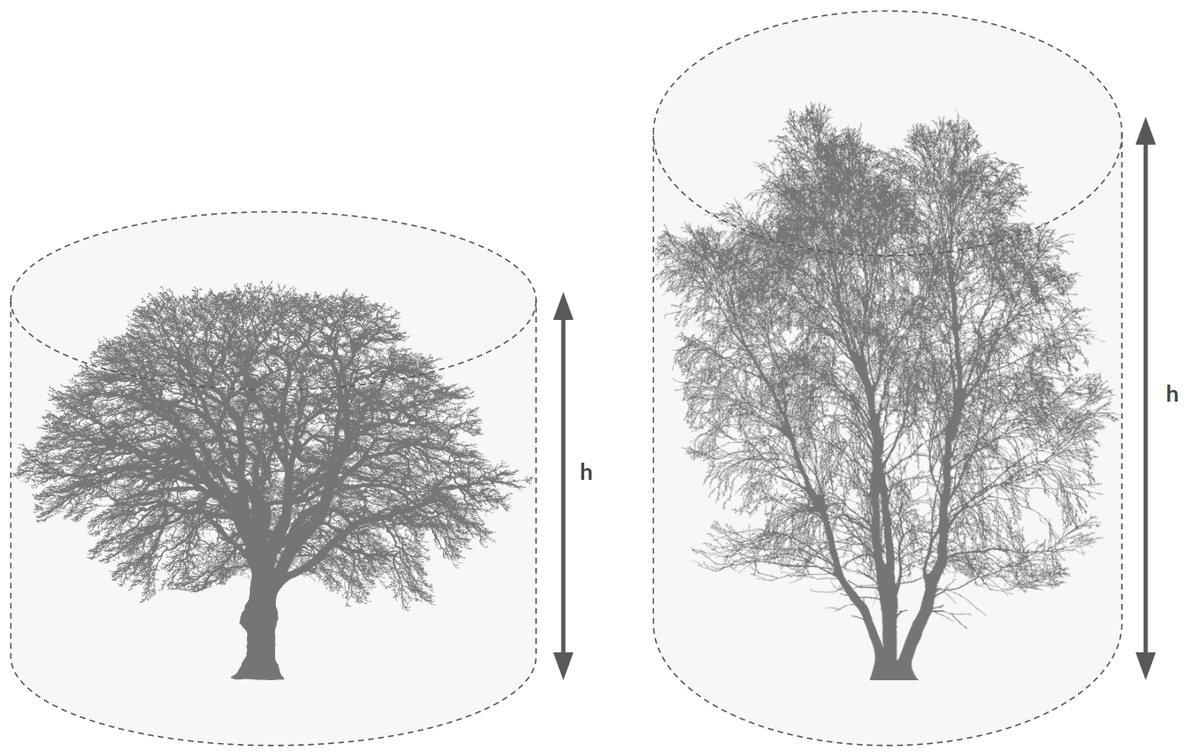
Leaf area density is calculated with respect to leaf area index \(LAI\) and height of the vegetation \(h\):
$$LAD=\frac{LAI}{h}\tag{5}$$
Read more about modeling tress in SimScale in our blog:
References
Last updated: May 25th, 2023
We appreciate and value your feedback.
What's Next
Advanced Modelling PWCpart of: Pedestrian Wind Comfort Analysis
Sign up for SimScale
and start simulating now