Atmospheric Boundary Layer for Pedestrian Wind Comfort Simulations
In the context of CFD modeling, an Atmospheric Boundary Layer (ABL) is an important aspect for modeling the flow around buildings, or for near-field dispersion problems. This can be relevant for many applications such as in Architecture, Pedestrian Wind Comfort (PWC), and Urban Planning. For a general description of the ABL, please refer to this article in our documentation.
This article explains how the ABL profile is generated with respect to the Wind Engineering Standards supported in the Pedestrian Wind Comfort simulation type in SimScale.
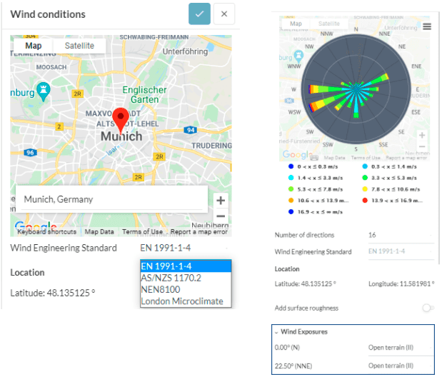
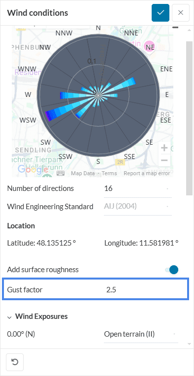
Before discussing the formulation utilized in generating the ABL, it is helpful to remember why and at which stage in a PWC simulation this is needed. When specifying the wind conditions you will be prompted with the choice of a wind engineering standard and a wind exposure category that will basically define how your ABL profile would look like coming from that particular direction of your terrain. See Figure 1 below for a snapshot of the interface illustrating this step.
1. Atmospheric Boundary Layer
The general formulations used to model the ground normal profiles such as velocity, turbulent kinetic energy (TKE) and the dissipation rate are based on [1,2,3].
1.1 Velocity Wind Profile
- The velocity profile utilizes the log-law and is as follows:
$$ u = \frac{u^*}{\kappa} \ln{\left(\frac{z – d + z_0}{z_0}\right)} \tag{1} $$
$$ v = 0 ;w = 0 $$
Important
The AS/NZS 1170.2 and the City of London (CoL) guidelines use a different approach to model the wind velocity profile, which is based on the Harris and Deaves boundary layer models. See section 2.2 and 2.4 for a description on the model used.
- The friction velocity \(u^*\) can be calculated as:
$$ u^* = \frac{u_{ref}\kappa}{\ln\frac{z_{ref} + z_{0}}{ z_{0}}}\tag{2} $$
Where
| $$u$$ | Ground-normal streamwise flow speed profile [\(m/s\)] |
| $$v$$ | Spanwise flow speed [\(m/s\)] |
| $$w$$ | Ground-normal flow speed [\(m/s\)] |
| $$u^*$$ | Friction velocity [\(m/s\)] |
| $$\kappa$$ | von Kármán constant = 0.41 |
| $$z$$ | Ground-normal coordinate component [\(m\)] |
| $$d$$ | Ground-normal displacement height [\(m\)] |
| $$z_{0}$$ | Aerodynamic roughness length [\(m\)] |
| $$u_{ref}$$ | Reference mean streamwise wind speed at \(z_{ref}\) [\(m/s\)] |
| $$z_{ref}$$ | Reference height being used in u∗ estimations [\(m\)] |
Displacement Height \((d)\)
According to [4] the displacement height \(d\) is relevant for flows over forests and cities. “The displacement height gives the vertical displacement of the entire flow regime over areas which are densely covered with obstacles such as trees or buildings.”
1.2 Turbulent Kinetic Energy, Dissipation Rate, and Specific Dissipation Rate Profiles
- Turbulent kinetic energy (TKE) profile:
$$ k = \frac{(u^*)^2}{\sqrt{C_{\mu}}} \sqrt{C_{1} \ln{\left(\frac{z – d + z_0}{z_0}\right)} + C_{2}}\tag{3}$$
- Turbulent kinetic energy dissipation rate:
$$ \epsilon = \frac{(u^*)^3}{\kappa ( z – d + z_0 )} \sqrt{C_{1} \ln{\left(\frac{z – d + z_0}{z_0}\right)} + C_{2}}\tag{4} $$
- The specific dissipation rate:
$$ \omega = \frac{u^*}{\kappa \sqrt{C_{\mu}}} \frac{1}{ z – d + z_0 }\tag{5} $$
Note
To produce a uniform TKE, the values for \(C_1\) and \(C_2\) are assumed to be by default 0 and 1, respectively. And the displacement height d is assumed to be 0.
- In general, through an experimental dataset for \(k\) and the constants \(C_1\) and \(C_2\), which are some curve-fitting coefficients, can be determined by non-linear fitting of equations 19 and 20 in [1]:
$$k = \sqrt{D_1 \ln{\left(\frac{z + z_0}{z_0}\right)} + D_2 }\tag{6} $$
- Where \(D_1\) and \(D_2\) includes \(C_1\) and \(C_2\) as follows:
$$D_1= \left(\frac{(u^*)^2}{\sqrt{C_{\mu}}}\right)^2 C_1 \tag{7} $$
$$D_2= \left(\frac{(u^*)^2}{\sqrt{C_{\mu}}}\right)^2 C_2 \tag{8} $$
Where
| $$ k $$ | Ground-normal turbulent kinetic energy (TKE) profile \([m^2/s^2]\) |
| $$\epsilon$$ | Ground-normal TKE dissipation rate profile \([m^2/s^3]\) |
| $$\omega$$ | Ground-normal specific dissipation rate profile \([m^2/s^3]\) |
| $$C_{\mu}$$ | Empirical model constant = 0.09 |
| $$C_1$$ | Curve-fitting coefficient for profiles |
| $$C_2$$ | Curve-fitting coefficient for profiles |
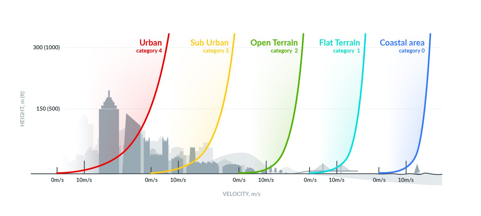
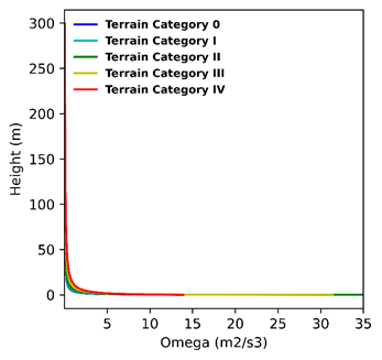
Figure 2 below, illustrates how the shape of the ABL profile changes with respect to the terrain category. The following section elaborates more on how these profiles differ for each wind engineering standard.
2. Wind Engineering Standards
When choosing one of the Wind Engineering Standards for your PWC simulation, the values of the variables in the ABL equations above vary depending on the exposure category. As shown above in Figure 2, the variability of the mean wind velocity depends on:
- The height above ground.
- The ground roughness of the terrain.
Each Wind Engineering Standard defines different values that associate best with the exposure category of that particular region.
Reference velocity and height
For generating the ABL profiles that follows, a reference velocity and a reference height of 10 \( m/s\) and 10 \( m\) had been used, respectively. In case of a custom terrain, there is not a single global \(z=0\) to use as a reference for the velocity profile, but it rather depends on the topology of the terrain.
Table 3 shows the six general exposure categories that are mostly used among wind engineering standards. Each wind engineering standard supplies different values of the ground surface roughness \(z_0\) either for all or some of these categories.
| General Exposure Category | Description |
| EC1 | City center with heavy concentration of tall building |
| EC2 | General urban area |
| EC3 | Suburban area |
| EC4 | Open terrain area |
| EC5 | Open lake or land with minimal obstruction |
| EC6 | Sea or coastal area |
Let’s discuss the Wind Engineering Standards supported within SimScale
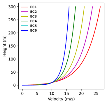
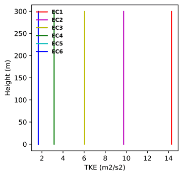
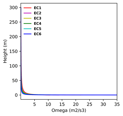
2.1 Eurocode en 1991-1-4:2005
The value of the aerodynamic roughness length \(z_0\) depending on the terrain category is shown in the table below. Moreover, the Eurocode does not provide values for the general exposure category EC1.
| Category | Description | $$z_0$$ [\(m\)] | Category name in Simscale Workbench |
| EC2 | General urban area | 1 | IV (Urban area) |
| EC3 | Suburban area | 0.3 | III ( Suburban area) |
| EC4 | Open terrain area | 0.05 | II (Open terrain) |
| EC5 | Open lake or land with minimal obstruction | 0.01 | I (Flat terrain) |
| EC6 | Sea or coastal area | 0.003 | 0 (Coastal area) |
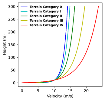
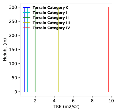
The ABL profiles for velocity, TKE, and specific dissipation rate which had been generated with a log law profile can be seen below for each terrain category:
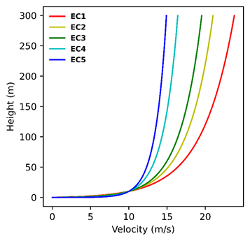
2.2 Australian/New Zealand Standard AS/NZS 1170.2:2011
The mean wind velocity profile is modeled using the Deaves and Harris approach. This model simulates a logarithmic atmospheric boundary layer profile as follows [6]:
$$ \bar{u} = \frac{u^*}{0.4} \left[\ln{\left(\frac{z}{z_0}\right)} + 5.75 \left(\frac{z}{z_g}\right) – 1.88 \left(\frac{z}{z_g}\right)^2 -1.33 \left(\frac{z}{z_g}\right)^3 +0.25 \left(\frac{z}{z_g}\right)^4 \right]\tag{9}$$
Where
| $$ \bar{u} $$ | Design hourly mean wind speed at height \(z\) \([m/s]\) |
| $$ z $$ | The distance or height above ground \(m\) |
| $$ z_0 $$ | Aerodynamic roughness length [\(m\)] |
| $$ z_g $$ | The gradient height = \(\frac{u^*}{B * f}\) |
| $$ f $$ | Coriolis Parameter = 0.0001 |
| $$B$$ | 6 |
\(u^*\), \(k\), and \(\omega\)
The formulations used to model these parameters are the same as in equations 2, 3, and 5, respectively.
Regarding the terrain categories in the AS/NZS standard there exists one difference to the Euro Code. The AS/NZS standard provides values for EC1 (heavy concentration of tall buildings) but not for EC2 (general urban area).
| Category | Description | $$z_0$$ [\(m\)] | Category name in Simscale Workbench |
| EC1 | City center with heavy concentration of tall buildings | 2 | City center |
| EC3 | Suburban area | 0.2 | Suburban area |
| EC4 | Open terrain area | 0.02 | Open terrain |
| EC5 | Open lake or land with minimal obstruction | 0.002 | Flat terrain |
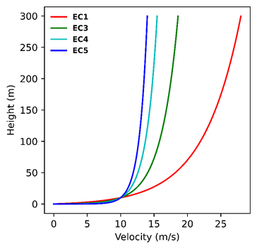
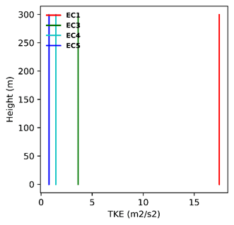
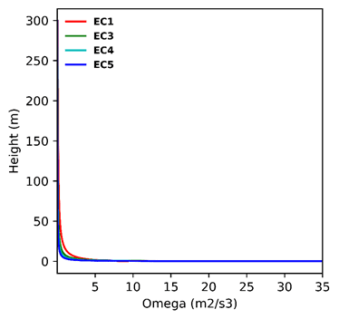
The following plots illustrate how the velocity, TKE, and specific dissipation rate looks like for each of the terrain categories of the AS/NZS defined above:
2.3 NEN8100 Dutch Standard
For the NEN8100 Dutch standard the following 6 terrain categories are available in SimScale and they are as follows:
| Category | Description | $$z_0$$ [\(m\)] | Category name in Simscale Workbench |
| EC1 | City center with heavy concentration of tall buildings | 2 | City center |
| EC2 | General urban area or forest | 1 | Urban or Forest |
| EC3 | Suburban area | 0.5 | Suburban |
| EC4 | Open terrain area (Rough) | 0.25 | Rough |
| EC5 | Open lake or land with minimal obstruction | 0.03 | Open |
| EC6 | Sea or coastal area | 0.0002 | Sea |
Due to the fact that the NEN8100 code utilizes a height of 60 \(m\) instead of 10 \(m\) as a reference height, a correction needs to be applied. More details can be found in the correction factors section in this documentation.
Below the ABL profile of velocity, TKE and specific dissipation can be seen:
2.4 City of London Wind Standard
The City of London wind standard models the variation of the mean and gust wind speed profiles based on the Harris and Deaves boundary layer models in the UK National Annex to the Eurocode.
$$ u (z) = \frac{u^*}{\kappa} \left[\ln{\left(\frac{z}{z_0}\right)} + 5.75 \left(\frac{z}{h}\right) – 1.88 \left(\frac{z}{h}\right)^2 -1.33 \left(\frac{z}{h}\right)^3 +0.25 \left(\frac{z}{h}\right)^4 \right]\tag{10}$$
Where
| \(h\) | Height of the neutral boundary layer = \( \frac{u^*}{B f}\) |
| \(f\) | Coriolis Parameter = 0.00011415 |
| \(B\) | 6 |
The model equation and the values for \(B\) and \(f\) provided above are based on [10,11,12].
\(u^*\) , \(k\), and \(\omega\)
The formulations used to model these parameters are the same as in equations 2, 3, and 5, respectively.
Furthermore, the roughness height values as a function of the exposure category for the London City wind standard are shown in the table below:
| Category | Description | $$z_0$$ [\(m\)] | Category name in Simscale Workbench |
| EC1 | City center with heavy concentration of tall buildings | 1 | Urban |
| EC2 | General urban area or forest | 0.5 | London City |
| EC3 | Suburban area | 0.3 | Suburban |
| EC4 | Open terrain area (Rough) | 0.05 | Open |
| EC5 | Open lake or land with minimal obstruction | 0.01 | Flat |
The ABL profiles depending on the values above are as follows:
2.5 AIJ (2004)
The main difference between the AIJ wind standard and the four standards discussed above is, that the AIJ ABL profile is based on Power law and not a Log law. A Gust factor also needs to be specified when defining wind conditions.
The roughness height values as a function of the exposure category for the AIJ (2004) wind standard are shown in the table below:
| Category | Description | alpha \(\alpha\) | \(z_0\) fitted at 10 \([m]\) | \(z_0\) fitted at 2 \([m]\) | Category name in Simscale Workbench |
| EC1 | An urban area densely populated with high-rise buildings (10 floors or more). | 0.35 | 4.44 | 2.335 | City Center (V, \(\alpha\) = 0.35 ) |
| EC2 | An urban area primarily composed of mid-rise buildings (4 to 9 floors). | 0.27 | 2.135 | 1.100 | Urban (IV, \(\alpha\) = 0.27) |
| EC3 | An area with numerous trees and low-rise buildings, or an area scattered with mid-rise buildings (4 to 9 floors). | 0.2 | 0.975 | 0.495 | Suburban (III, \(\alpha\) = 0.2) |
| EC4 | An area with obstacles similar to crops, like pastoral regions or grasslands, and areas scattered with trees and low-rise buildings. | 0.15 | 0.485 | 0.240 | Open (II, \(\alpha\) = 0.15) |
| EC5 | An area with few obstacles, such as a coastline or the surface of a lake. | 0.1 | 0.215 | 0.100 | Flat (I, \(\alpha\) = 0.1) |
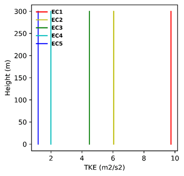
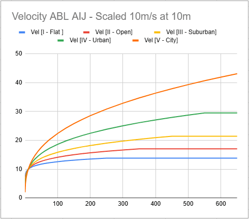
Inlet profiles for the AIJ (2004) can be found below:
Velocity Profile
Consistent with the other Wind Engineering Standards, SimScale runs the CFD analysis with a fixed reference speed of 10 \(m/s\) at the reference height of 10 \(m\).
To be consistent and to ensure numerical stability SimScale does not use the blending height \(z_b\) values provided by AIJ, but keeps them all at 0 \(m\) and has a full power law profile down to 0 \(m\).
$$U_z = 10 \left(\frac{z_{min}}{10}\right)^\alpha …….. z < z_{min} \tag{11.1}$$
$$U_z = 10 \left(\frac{z}{10}\right)^\alpha …….. z_{min} < z < z_G \tag{11.2}$$
$$U_z = 10 \left(\frac{z_G}{10}\right)^\alpha …….. z >= z_G \tag{11.3}$$
where \(\alpha\) and \(z_G\) are given in the table below.
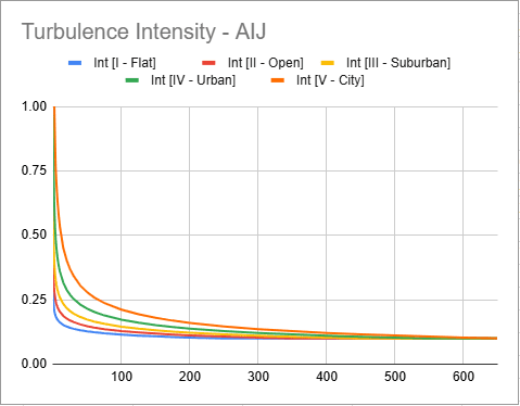
Turbulent Intensity Profile
$$I_z = 0.1 \left(\frac{z_{min}}{z_G}\right)^{-\ \alpha -\ 0.05} ………z < z_{min} \tag{12.1}$$
$$I_z = 0.1 \left(\frac{z}{z_G}\right)^{-\ \alpha -\ 0.05} ………z_{min} < z < z_G \tag{12.2}$$
$$I_z = 0.1 ……. z >= z_G \tag{12.3}$$
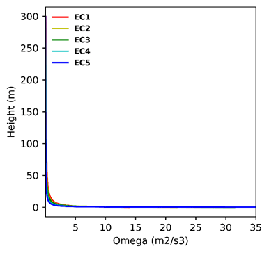
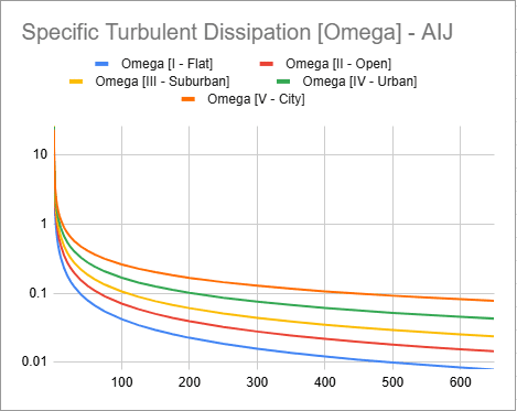
Omega (Specific Turbulent Dissipation) profile
We can derive the Omega profile from the inlet form the TKE, velocity and viscosity data using the following formula (see AIJ doi:10.1016/j.jweia.2008.02.058):
$$\omega(z) = \frac{\epsilon(z)}{C_{\mu}\ k(z)} $$
$$\epsilon(z) = C_{\mu}^{1/2}\ k(z)\ \frac{U_{ref}}{z_{ref}} \alpha \left(\frac{z}{z_{ref}}\right)^{(\alpha -\ 1)} $$
Combining both formulas, we get:
$$\omega(z) = C_{\mu}^{-1/2}\ \frac{U_{ref}}{z_{ref}} \alpha \left(\frac{z}{z_{ref}}\right)^{(\alpha – 1)} \tag{13}$$
Adding in the reference height of 10 \(m\) and reference velocity of 10 \(m/s\) we get:
$$ \omega(z) = C_{\mu}^{-1/2} \alpha \left(\frac{z}{10}\right)^{(\alpha – 1)} \tag{14}$$
3. Evaluation of the Pedestrian Wind Comfort Criteria
To assess a PWC study, three different types of information are needed:
- Statistical meteorological data
- Aerodynamic information
- A comfort criterion
The transformation of the statistical meteorological data to the location of interest at the building site is realized through the aerodynamic information, which is split into two parts:
- Terrain contribution: Accounts for the change in terrain between the meteorological site and a location near or at the site of the building.
- Design contribution: Accounts for the change in wind statistics due to local urban configuration.
Understanding this is the basis for the evaluation of pedestrian comfort, to do so, the local wind velocity needs to be related to the weather station data in order to obtain the probability of the local wind speed exceeding the threshold wind speeds defined by the comfort criterion.
The relation between the measured wind speed at the meteorological station \(u_{meteo}\) to the local wind speed \(u_{loc}\) is defined as the “wind amplification factor”:
$$ \gamma = \frac{u_{loc}}{u_{meteo}}\tag{15} $$
This can be split up in two components:
$$ \gamma = \frac{u_{loc}}{u_{meteo}} = \frac{u_{loc}}{u_0} * \frac{u_0}{u_{meteo}} \tag{16} $$
- \(\frac{u_{loc}}{u_0}\) : Local contribution of the topography close to the building (Design contribution of the aerodynamic information; transformation of \(u_0\) to \(u_{loc}\)).[9]
- \(\frac{u_{0}}{u_{meteo}}\) : Corrective factor for the weather station wind data. (Terrain contribution of the aerodynamic information; transformation of \(u_{meteo}\) to \(u_0\)).[9]
The figure below illustrates this further. (Note: \(u_{pot}\) refers to \(u_{meteo}\) in the figure)
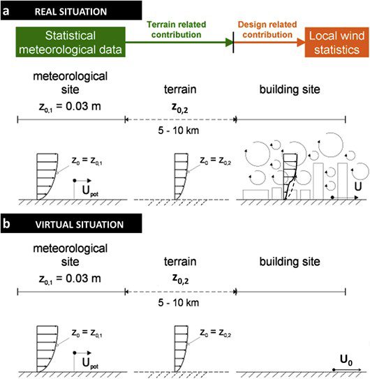
From the CFD analysis we get the first part \( \frac{u_{loc}}{u_0}\) directly. However, the correction of the weather station data \(\frac{u_0}{u_{meteo}}\) requires additional effort and calculations, which can differ between each wind engineering standard.
4. Wind Comfort Criteria and the Weibull Distribution
The wind comfort standards define limits that are related to the threshold local air speeds based on the type of activity. These limits cannot be exceeded for more than a specified percentage of time in a year.
For example, the table below illustrates the comfort levels based on the Lawson comfort criteria:
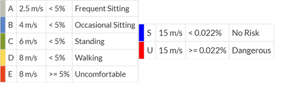
A meteorological wind station provides a discrete set of wind data, therefore in order to evaluate the probabilities of exceedance at any given threshold speed, the discrete set of data is fitted into a continuous one by the mean of a Weibull probability distribution.
Moreover, from the CFD simulation, we receive the locally measured wind speeds, and by using them with the combination of the parameters inside the Weibull probability distribution function, the probability of exceeding a certain wind speed at a specific location can be obtained. The City of London guidelines defines the Weibull function as:
$$ f(x) = P . e^{(-\frac xc)^k} \tag{17} $$
Where
| \(f\) | Frequency |
| \(P\) | The probability that the wind will approach from a certain direction |
| \(x\) | A given wind speed [m/s] |
| \(c\) | Scale factor |
| \(k\) | Shape factor |
Now we understand how the comfort criteria is evaluated. Nevertheless, a correction to the wind speed value inside the Weibull function is necessary to take into account the aerodynamic information discussed earlier in the preceding section. The correction values are incorporated in terms of the wind amplification factor inside equation 15, by multiplying with the scale factor \(c\) inside the Weibull probability distribution function. (refer to the example section below for an overview of the calculation method)
5. Correction Factors
Since each wind engineering standard utilizes slightly different methods in conducting the design one has to account for these variations through correction factors. Corrections for the averaging time of the velocity or terrain exposure correction factor are some examples of possible corrections to be carried out.
5.1 Eurocode
For the EU standard the logarithmic boundary profile is valid until a maximum height of \(z_b\) = 200 \(m\), so we are also assuming this height as the blending height for all categories. This leads to the following :
Blending Height
Blending height refers to the height where the terrain effects are negligible and irrespective of the terrain the same speed is present. Which yields:
\(u_{meteo} \ (z_b) = u_0 \ (z_b)\)
$$ \gamma = \frac{u_{loc}}{u_{meteo}} = \frac{u_{loc}}{u_0} * \frac{u_0}{u_{meteo}} $$
The term \( \frac{u_{loc}}{u_0}\) can be calculated directly from the CFD simulation, where \(u_{loc}\) represents the local measured velocity at the location of interest, and \(u_0\) is the velocity at defined reference height 10 \(m/s\) at 10 \(m \) height.
$$ \frac{u_0}{u_{meteo}} = \frac{u_0 (z_b= 200 m)} {u_{meteo} (z_b= 200 m)}\tag{18} $$
$$ \frac{u_0}{u_{meteo}} = \frac{{u_0}^* \ln{ |\frac{z_b}{{z_{0}}}+ 1 }|} {{u_{meteo}}^* \ln{ |\frac{z_b}{{z_{0}}_{meteo}}+ 1 }| } \tag{19}$$
Inserting the formula of \(u^*\) into the equation above and centering it at 1 for EC4 (the terrain category of the meteorological station) results in:
$$ \frac{u_0}{u_{meteo}} = \frac{ln{ |\frac{z_{ref}}{{z_{0}}}+ 1 }|} {ln{ |\frac{z_{ref}}{{z_{0}}_{meteo}}+ 1 }| } * \frac{ln{ |\frac{z_{b}}{{z_{0}}_{meteo}}+ 1 }|} {ln{ |\frac{z_b}{{z_{0}}}+ 1 }|} \tag{20}$$
$$ \frac{u_0}{u_{meteo}} = \frac{ln{ |\frac{10}{{z_{0}}}+ 1 }|} {ln{ |\frac{10}{{z_{0}}_{meteo}}+ 1 }| } * \frac{ln{ |\frac{200}{{z_{0}}_{meteo}}+ 1 }|} {ln{ |\frac{200}{{z_{0}}}+ 1 }|} \tag{21}$$
The evaluation of the expression above for the different terrain categories yields the following correction factors as shown in the table below:
| Category | EC6 | EC5 | EC4 | EC3 | EC2 |
| Description | Coastal Area | Flat Terrain | Open Terrain | Suburban Area | Urban Area |
| Roughness \((z_0 [m])\) | 0.003 | 0.01 | 0.05 | 0.3 | 1 |
| Correction factor \((\frac{u_0}{u_{meteo}})\) | 1.14 | 1.09 | 1 | 0.85 | 0.707 |
5.2 AS/NZS
Here the correction is directly related to the difference between the terrain category at which the meteorological data had been calculated and the terrain category at or near the building site.
As mentioned earlier, in order to evaluate the PWC we need to calculate the wind amplification factor which was split into two parts (see equations 15 and 16 above):
- \(\frac{u_{loc}}{u_0}\)
- \(\frac{u_{0}}{u_{meteo}}\)
Since the meteorological data was calculated on terrain EC4 (open area terrain), it should have a factor of 1.0 (meaning that no correction is needed if the terrain category of the site of interest is also EC4).
The meteorological data is measured at 10 \(m\) height, and based on that one can read the values of the velocity profile multipliers for each terrain category (see table 5 above for the description of each terrain category) from the 1989 AS/NZS standard as :
- EC5 : 0.71
- EC4 : 0.60
- EC3 : 0.44
- EC1 : 0.35
Finally, we get the factor for each terrain category by centering the sequence above at 1.0 for EC4:
| Category | EC5 | EC4 | EC3 | EC1 |
| Description | Flat Terrain | Open Terrain | Suburban Area | City Center |
| Roughness \((z_0 [m])\) | 0.002 | 0.02 | 0.2 | 2 |
| Correction factor \((\frac{u_0}{u_{meteo}})\) | 1.183 | 1.0 | 0.733 | 0.583 |
5.3 NEN8100
The meteorological data for the NEN8100 wind standard is already corrected to the local roughness directly by the NEN8100 code. Therefore, no direct exposure correction needs to take place.
However, the wind speed data for NEN8100 is defined at 60 \(m\) height but in the context of the framework followed by SimScale a 10 \(m\) height for the reference velocity is utilized. Hence, a correction is needed to scale down to the 10 \(m\) reference height.
As we have,
$$ \frac{u_0}{u_{meteo}} = \frac{{u_0}^* \ln{ |\frac{10}{z_0}+ 1|}} {{u_{meteo}}^* \ln{ |\frac{60}{z_0}+ 1|}} = \frac{\ln{ |\frac{10}{z_0}+ 1|}} {\ln{ |\frac{60}{z_0}+ 1|}} \tag{22}$$
| Category | EC6 | EC5 | EC4 | EC3 | EC2 | EC1 |
| Description | Sea | Open | Rough | Suburban | Urban or Forest | City Center |
| Roughness \((z_0 [m])\) | 0.0002 | 0.03 | 0.25 | 0.5 | 1 | 2 |
| Correction factor$$(\frac{u_0}{u_{meteo}})$$ | 0.81910 | 0.76461 | 0.67707 | 0.63483 | 0.58331 | 0.52177 |
Note
These categories are not fully fixed by NEN8100, they are rather fitted to cover best the roughness appearing in the related NPR 6097 standard.
5.4 City of London Wind Standard
For the CoL standard, the weather data is given directly as Weibull coefficients and they relate to a reference height of 120 \(m\). No exposure correction is needed if the default CoL exposure (\(z_0\)=0.5 \(m\)) is used.
The relation between the measured wind speed at the inlet reference velocity \(u_{120m}\) to the local wind speed \(u_{loc}\) is defined as the “wind amplification factor” as stated before.
$$ \gamma = \frac{u_{loc}}{u_{120}} = \frac{u_{loc}}{u_0} * \frac{u_0}{u_{120}} $$
The first one being the local contribution of the topography close to the building, whereas the second part is the corrective factor for the wind data, which is usually given for a specific reference terrain category (here “London City” terrain with 0.5 \(m\) roughness).
From the CFD analysis we get the first part \(\frac{u_{loc}}{u_0}\) directly. On the other hand, the correction of the weather data \(\frac{u_0}{u_{120}}\) , requires some additional effort.
The atmospheric boundary layer profile is valid until a max height of \(z_g\) = \(h\) (gradient height from Deaves and Harris model), so we are assuming for consistency reasons that this height is also the blending height (using always the lower gradient height of the two categories in transition).
| Category | EC5 | EC4 | EC3 | EC2 | EC1 |
| Description | Flat | Open | Suburban | London City | Urban |
| Roughness \((z_0 [m])\) | 0.01 | 0.05 | 0.3 | 0.5 | 1 |
| Correction factor$$(\frac{u_0}{u_{120}})$$ | 1.17 | 1.14 | 1.05 | 1 | 0.87 |
5.5 AIJ (2004)
The calculation for the Speedup factor gamma for the AIJ (2004) standard is given by:
$$ \gamma= \frac{u_{0}}{u_{meteo}} $$
Where a 10 \(m\) height for the reference velocity is utilized.
We assume the same velocity at the gradient height. For consistency, we use the lower of the two gradient heights as the intersection point.
| Category | EC5 | EC4 | EC3 | EC2 | EC1 |
| Description | Flat (I, \(\alpha\) = 0.1) | Open (II, \(\alpha\) = 0.15) | Suburban (III, \(\alpha\) = 0.2) | Urban (IV, \(\alpha\) = 0.27) | City Center (V, \(\alpha\) = 0.35) |
| Blending height \((z_b [m])\) | 5 | 5 | 5 | 10 | 10 |
| Gradient height \((z_G [m])\) | 250 | 350 | 450 | 550 | 650 |
| Correction factor wrt EC4 $$(\frac{u}{u_meteo})$$ | 1.175 | 1 | 0.837 | 0.653 | 0.491 |
6. Application Example Using the AS/NZS 1170 Standard
This example demonstrates the calculation procedure for the comfort criteria. The necessary inputs for this are:
- Meteorological data 🡪 Wind Rose
- Wind exposure 🡪 Wind standard and terrain category for each direction.
- CFD simulation results 🡪 Wind speeds at pedestrian level (1.5 \(m\) ~ 1.75 \(m\)) for each of the analyzed wind directions.
The steps for calculation are as follows:
- Derive the Weibull distribution.
- Compute local contribution (speed up factor) \(\frac{u_{loc}}{u_0}\) from CFD results.
- Compute the contribution due to wind exposure correction \(\frac{u_0}{u_{meteo}}\).
- Calculate the wind amplification factor γ.
- Compute Comfort Criteria (NEN8100) according to threshold speeds and probability of exceedance.
Step 1:
- In this step we only need to specify the wind direction and setup the equation for following analysis.
- Corresponding to the location we are analyzing we can obtain the wind rose. The wind rose would indicate which wind direction is the most critical. Based on this we can calculate the probability of wind coming from a certain direction \(P\).
$$ f(x) = P . e^{(-\frac uc)^k} $$
Step 2:
- From the CFD simulation we obtain the average velocities at pedestrian level for a specific direction. For demonstration purposes let’s assume that at the point of interest a velocity of 8 \(m/s\) had been calculated.
- Our reference velocity \(u_0\) is equal to 10 \(m/s\) at a reference height of 10 \(m\).
- The local speed up factor can be then calculated as:
$$\frac{u_{loc}}{u_0}= \frac{8 \ m/s} {10 \ m/s} = 0.8 $$
- Be aware, that this value is unique to that particular point of interest and is dependent on the wind direction used in this analysis.
Step 3:
- For this example we assume that the terrain where the wind is coming from corresponds to exposure category 4 in the AS/NZS standard.
- Accordingly, from Table 13 in the AS/NZS correction factor section above, we can obtain our correction factor as:
$$ \frac{u_0}{u_{meteo}} = 0.58 $$
- Please note that this value is constant for all points in the simulation, but it depends on the wind direction. The reason being each wind direction might correspond to a different terrain category.
Step 4:
- The wind amplification factor can be calculated as:
$$ \gamma= \frac{u_{loc}}{u_{meteo}} = 0.8 * 0.58=0.46 $$
- One way to interpret this value can be: Assume that a wind speed of 1 \(m/s\) is measured at the weather station from a specific wind direction, then we approximate the local average wind speed at the pedestrian level as 0.46 \(m/s\)
Step 5:
- Having derived the Weibull distribution from the wind rose data, we can compute the probability of the wind exceeding a threshold of 5 \(m/s\) at the point of interest for a wind coming from a specific wind direction \((dir)\):
$$ f(dir , u > 5 m/s ) = P_{dir} . e^{(-\frac{u}{c})^k} $$
$$ = P_{dir} . e^{-\left(\frac{5}{0.46c_{dir}}\right)^{k_{dir}}} $$
$$ = P_{dir} . e^{\left(-\frac{10.87}{c_{dir}}\right)^{k_{dir}}} $$
- Let’s assume that the probability of wind coming from direction dir is 10% and the probability that the wind coming from that direction actually exceeds 10.87 \(m/s\) is 15%. This means we have a 1.5% chance of a wind at location x coming from direction dir and exceeding 5 \(m/s\).
- If we assume all n wind directions are the same, and all have the same amplification factor, probability distribution, and probability of the wind direction to appear, we will have in total a 15% chance of locally exceeding 5 \(m/s\).
For the NEN8100 standard this would mean we are in category D (Walking Fast).
For Lawson we would need to check the exceedance probabilities for 1.8 \(m/s\), 3.6 \(m/s\), 5.3 \(m/s\), and 7.6 \(m/s\) – so with these numbers we would definitely not make categories A – C for Lawson and might even fail D as the threshold for that is 2%.
Related Articles
- How Does Surface Roughness Affect PWC Results?
- How Does PWC Analysis Deal With Complex Geometry at the Boundary?
References
- Hargreaves, D. M., & Wright, N. G. (2007). On the use of the k–ε model in commercial CFD software to model the neutral atmospheric boundary layer. Journal of wind engineering and industrial aerodynamics, 95(5), 355-369.
- Yang, Y., Gu, M., Chen, S., & Jin, X. (2009). New inflow boundary conditions for modelling the neutral equilibrium atmospheric boundary layer in computational wind engineering. Journal of Wind Engineering and Industrial Aerodynamics, 97(2), 88-95.
- Richards, P. J., & Norris, S. E. (2011). Appropriate boundary conditions for computational wind engineering models revisited. Journal of Wind Engineering and Industrial Aerodynamics, 99(4), 257-266.
- Emeis, S. (2018). Wind energy meteorology: atmospheric physics for wind power generation. Springer.
- EN 1991-1-4: Eurocode 1: Actions on structures – Part 1-4: General actions – Wind actions. . EN 1991-1-1-4. (n.d.).
- AS/NZS- 1170.2:2011 – https://www.standards.govt.nz/shop/asnzs-1170-22011/
- NEN8100 standard – https://www.nen.nl/en/nen-8100-2006-nl-107592
- London City Wind Standard – https://in2.iehttps://frontend-assets.simscale.com/media/2019/11/city-of-london-wind-microclimate-guidelines.pdf
- Blocken, B., Stathopoulos, T., & Van Beeck, J. P. A. J. (2016). Pedestrian-level wind conditions around buildings: Review of wind-tunnel and CFD techniques and their accuracy for wind comfort assessment. Building and Environment, 100, 50-81.
- Cook, N. J. (1997). The Deaves and Harris ABL model applied to heterogeneous terrain. Journal of wind engineering and industrial aerodynamics, 66(3), 197-214.
- Drew, D. R., Barlow, J. F., & Lane, S. E. (2013). Observations of wind speed profiles over Greater London, UK, using a Doppler lidar. Journal of Wind Engineering and Industrial Aerodynamics, 121, 98-105.
- Kent, C. W., Grimmond, C. S. B., Gatey, D., & Barlow, J. F. (2018). Assessing methods to extrapolate the vertical wind-speed profile from surface observations in a city centre during strong winds. Journal of Wind Engineering and Industrial Aerodynamics, 173, 100-111.
Last updated: July 29th, 2025
Did this article solve your issue?
How can we do better?
We appreciate and value your feedback.


