Documentation
This validation case belongs to fluid dynamics. The aim of this validation case is to validate the Conjugate heat transfer (CHT) analysis implemented in SimScale.
The simulation results of SimScale were compared to the results presented in the study titled “Unshrouded Plate Fin Heat Sinks for Electronics Cooling: Validation of a Comprehensive Thermal Model and Cost Optimization in Semi-Active Configuration”\(^1\) written by L. Ventola, G. Curcuruto, et. al.
The geometry used for the case has three regions, which are as follows:
The length of the fluid region upstream of the heat sink is 6 times the length of the heat sink \((L)\) and the fluid region length downstream is 15 times \(L\) visualized in the figure below:
The model of the heat sink with its dimensions can be seen in the figure and table below:
| Dimension \([mm]\) | Value |
| h (height) | 21.8 |
| W (width) | 41.4 |
| L (length) | 57.2 |
| t_b (base height) | 8.4 |
| t (thickness of fin) | 1 |
| p (spacing between adjacent fins) | 2.1 |
| N (number of fins) | 14 |
The heat source is a chip with the dimensions shown in the table below and has a contact surface area \((A_s)\) with a heat sink of 1.555 \(cm^2\).
| Dimension \([mm]\) | Value |
| a | 15.5 |
| b | 10 |
| c | 4.5 |
| d | 9 |
| e | 1.3 |
Chip Model
STP130NS04ZB by STMicroelectronics
Tool Type: OpenFOAM®
Analysis Type: Conjugate Heat Transfer
Mesh and Element Types:
The mesh was generated using the Standard meshing algorithm. The following table provides the details of the mesh:
| Mesh Type | Number of Cells | Element Type |
| Standard | 603883 | 3D Polyhedral |
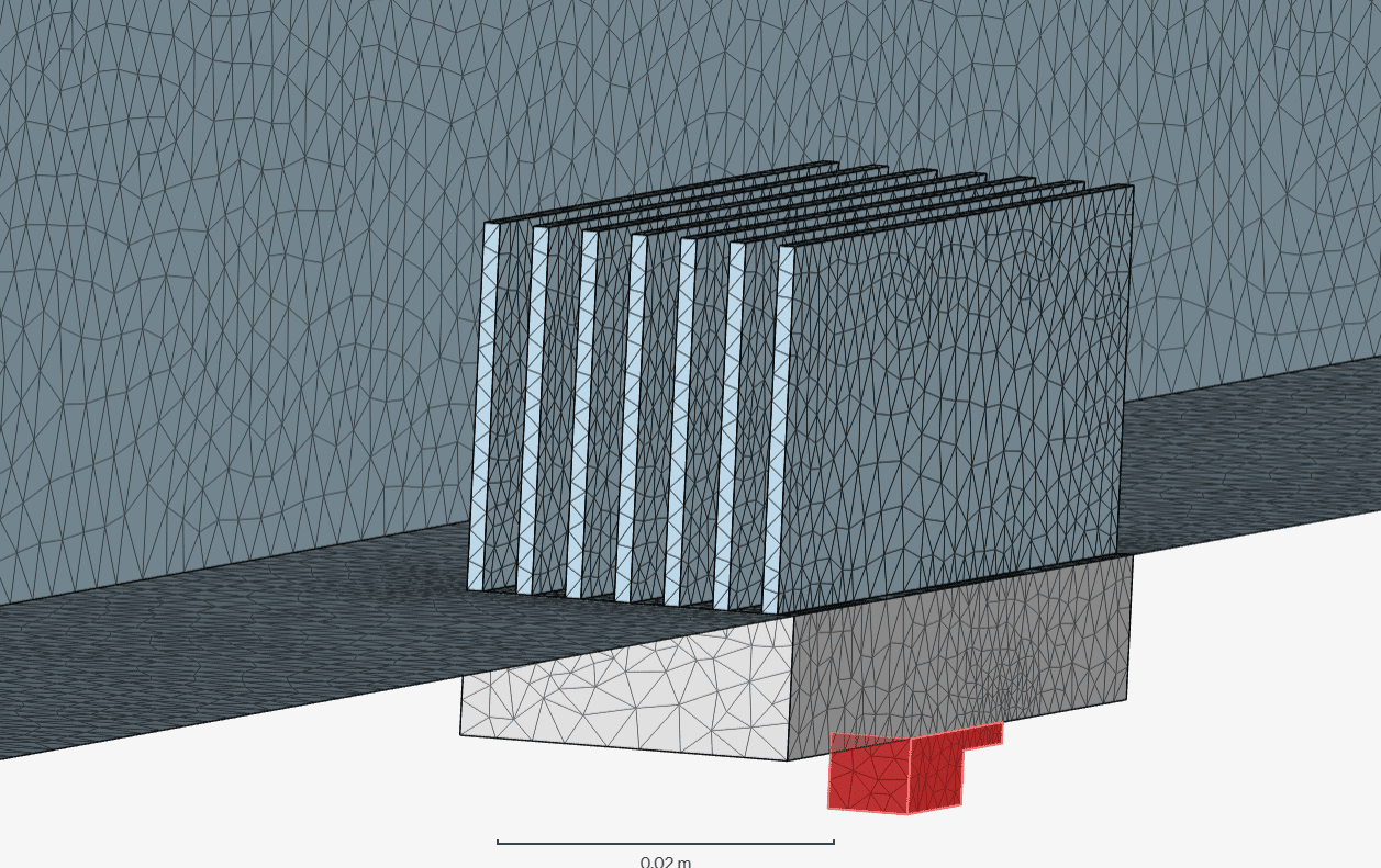
A region refinement was added to the heat source, heat sink, and the area close to the heat sink to be able to accurately capture the features of the heat sink as well as the wake region. In order to reduce the cell count and therefore decrease the run time, a symmetry plane in the XZ-Plane is used. A local element refinement was further used to increase the fineness around the fins of the heat sink. The mesh of the heat sink, heat source, and symmetry plane can be seen in the figure below:
Material:
$$\kappa_{hs} = \frac{\frac{1}{2}a}{R_{jc}A_s} \tag{1}$$
where:
Initial Conditions:
The velocity \((U)\) and temperature \((T)\) are given an initial condition, based on the experimental results, the same as for the boundary conditions to allow for faster convergence of the simulation.
Boundary Conditions:
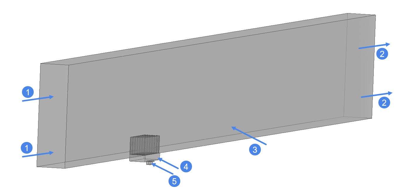
| Surface | Boundary Condition |
| 1 | Volumetric Flow Inlet |
| 2 | Pressure Outlet |
| 3 | Symmetry Plane |
| 4 | Symmetry Plane Heat Sink |
| 5 | Symmetry Plane Chip |
The simulation was run with 7 different volumetric flow rates with each volumetric flow rate having its corresponding inlet temperature and heat source, as seen in the table below:
| Approach (Inlet) Velocity \([m/s]\) | Volumetric flow rate \(\dot{U}\,[m^3/s]\) | \(T\,[K]\) | Absolute Power Source (chip) \([W]\) | Pressure Outlet \([Pa]\) | Walls | Heat Sink |
| 5.47 | 0.027 | 296.9 | 56.64 | 0 | No-slip | No-slip |
| 7.03 | 0.0352 | 297.4 | 71.4 | 0 | No-slip | No-slip |
| 8.59 | 0.04295 | 297.9 | 82.36 | 0 | No-slip | No-slip |
| 9.96 | 0.0498 | 298.3 | 87.32 | 0 | No-slip | No-slip |
| 11.23 | 0.0562 | 298.9 | 85.07 | 0 | No-slip | No-slip |
| 12.50 | 0.062 | 299.3 | 76.3 | 0 | No-slip | No-slip |
| 13.57 | 0.06783 | 299.6 | 60.24 | 0 | No-slip | No-slip |
Note
The walls of the heat sink were automatically assigned as walls with temperature as zero gradient. This assignment cannot be seen under Boundary conditions in the attached project.
The overall heat resistance between the heat source and the ambient air (heat sink) \((R_{ja})\) as calculated in the analytical and experimental results from the reference study\(^1\) are explained as follows. The complete array of thermal resistances between the heat source and the ambient air can be seen in the figure below:
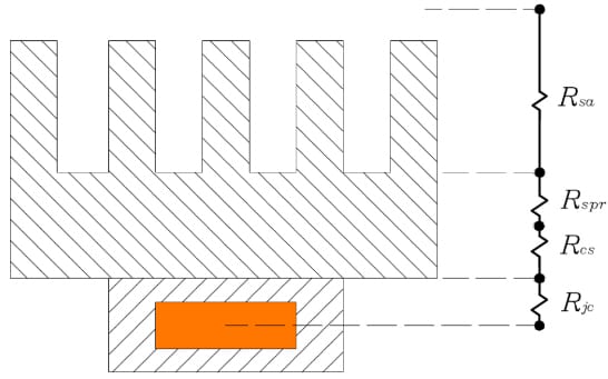
The analytical solution for the junction-to-air thermal resistance is given by:
$$R_{ja,t} = R_{jc}+R_{cs}+R_{sa}+R_{spr} \tag{2}$$
where:
The experimental solution is gained by doing an experiment with the scheme explained in the figure below:
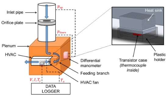
The air at ambient temperature flows into the rig and the airflow is measured with an orifice plate method where the orifice plate is in the inlet pipe. Then, the air flows into a plenum chamber and finally passes through a feeding branch, and enters the HVAC. The HVAC fan flows the air through the experimental rig where the heat sink is placed.
The transistor voltage drop (\(V\)), electric current (\(I\)), junction temperature (\(T_j\)) and the temperature of air approaching the heat sink (\(T_a\)) are measured with a GL220 data logger (Graphtec™ Digital Solutions, Plano, TX, USA)\(^1\). The junction temperature (\(T_j\)) is measured at the interface between the transistor and the heat sink and the approaching air temperature (\(T_a\)) is measured at the inlet of the HVAC. Finally, the overall junction-to-air thermal resistance is calculated with the formula below:
$$R_{ja,e} = \frac{T_j-T_a}{P} \tag{3}$$
Where:
The junction-to-air thermal resistance (\(R_{ja}\)) obtained from SimScale was calculated using the equation below:
$$R_{ja,s} = \frac{T_{j,s}-T_a}{P} \tag{4}$$
Where:
The comparison of the junction-to-air thermal resistance (\(R_{ja}\)) between the simulation results and the results in the reference study is given in Table 5 and Figure 9:
| Approach (Inlet) Velocity \([m/s]\) | Volumetric Flow Rate \(\dot{U}\,[m^3/s]\) | \(T_a\) \([K]\) | P \([W]\) | \(T_{j,e}\) \([K]\) | \(T_{j,s}\) \([K]\) | \(R_{ja,t}\) \([K/W]\) | \(R_{ja,e}\) \([K/W]\) | \(R_{ja,s}\) \([K/W]\) | Error – Simulation to Analytical [%] | Error – Simulation to Experiment [%] |
| 5.47 | 0.027 | 296.95 | 56.64 | 371.25 | 370.84 | 1.203 | 1.312 | 1.304 | 8.44 | -0.567 |
| 7.03 | 0.0352 | 297.35 | 71.4 | 384.15 | 384.03 | 1.142 | 1.216 | 1.214 | 6.30 | -0.164 |
| 8.59 | 0.04295 | 297.95 | 82.36 | 391.85 | 392.89 | 1.1 | 1.140 | 1.152 | 4.79 | 1.11 |
| 9.96 | 0.0498 | 298.25 | 97.32 | 395.05 | 406.4 | 1.071 | 1.109 | 1.11 | 3.76 | 0.205 |
| 11.23 | 0.0562 | 298.95 | 85.07 | 391.15 | 391.146 | 1.05 | 1.084 | 1.083 | 3.215 | -0.02 |
| 12.50 | 0.062 | 299.25 | 76.3 | 377.45 | 380.435 | 1.031 | 1.024 | 1.064 | 3.20 | 3.908 |
| 13.57 | 0.06783 | 299.65 | 60.24 | 357.55 | 362.87 | 1.017 | 0.961 | 1.049 | 3.19 | 9.205 |
![conjugate heat transfer validation Heat Sink Thermal Resistance [K/W]](https://frontend-assets.simscale.com/media/2025/06/image-40.png)
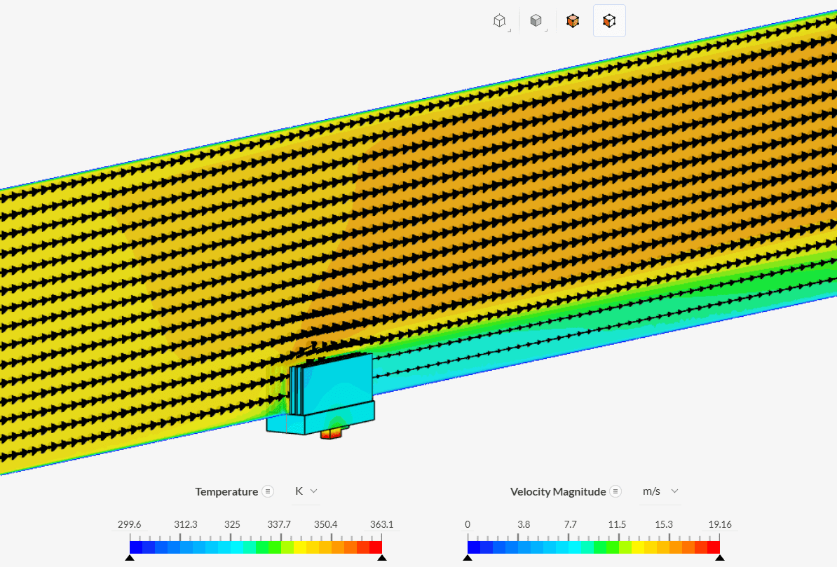
The temperature distribution on the heat sink and velocity distribution on chip obtained from the simulation when the approach velocity is 13.57 \(m/s\) are as below:
Note
If you still encounter problems validating you simulation, then please post the issue on our forum or contact us.
Last updated: February 8th, 2026
We appreciate and value your feedback.
Sign up for SimScale
and start simulating now