Documentation
This validation case belongs to fluid dynamics using Pacefish®, which is developed by Numeric Systems GmbH\(^3\). The aim of this test case is to validate the following parameters on a building with balconies, using the Lattice Boltzmann model:
A series of experiments on a 1:400 scale model of a high-rise building with balconies at its facade was performed by T. Stathopoulos and X. Zhu \(^2\), using as a parameter of interest the mean surface pressure on the facade for different wind directions. The measurements were performed in the atmospheric boundary layer open-circuit wind tunnel of the Center for Building Studies at Concordia University in a wind-tunnel with a test section of 12.2 \(m\) length and a cross-section of 1.8 x 1.8 \(m^2\).
The wind tunnel results were recreated with the ANSYS CFD software in a paper by X. Zheng a, H. Montazeri and B. Blocken , titled ” CFD simulations of wind flow and mean surface for buildings with balconies: Comparison of RANS and LES”\(^1\) showcasing the capability of CFD solvers in matching the experimental values for Wind Loading.
The geometry used for the case is as follows:
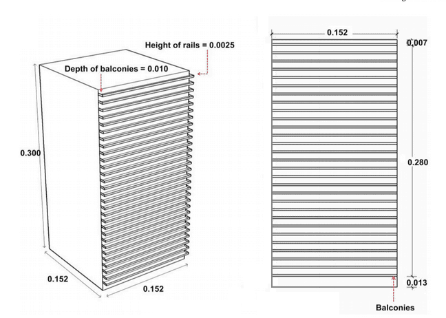
It is a 1:400 scaled model of a real high-rise building with 30 levels of balconies.
The solver that is used for this validation is the Lattice Boltzmann by Pacefish®, a fast method for incompressible analysis of robust models, using GPUs for the simulation.
For this validation case, the Pacefish® turbulence model chosen is the Improved Delayed Detached Eddy Simulation model (IDDES). It is a hybrid LES-URANS model that has an advantage of switching between the Large Eddy Simulation (LES) at regions where the Mesh Lattice is fine enough and the RANS model where the solid boundaries are present to well resolve the boundary layers, achieving an optimum between both worlds.
The approach-flow mean velocity and longitudinal turbulence intensity profiles were measured at the center of the turntable in the empty tunnel (i.e. without the building model present), and hence represent the so-called incident profiles. The profiles (shown in Figure 1) reproduced an open country terrain exposure with aerodynamic roughness length of 0.0001 m (model scale, corresponding to 0.04 m at full scale), and the reference wind speed \(U_{ref}\) of approximate 14 m/s at gradient height (Hg 1⁄4 0.625 m, corresponding to 250 m at full scale).
In order to match the velocity conditions of the experimental and CFD data from the paper, a profile was created for the velocity, as defined in the paper:
$$U = \frac{u_{ABL}^{*}}{k}\ln \left ( \frac{z+z_{o}}{z_{o}} \right )\tag{1}$$
where:
| \(u_{ABL}^{*}\) | Measured mean wind speed reference value. | 0.7 \(m/s\) |
| \(k\) | The von Karman constant. | 0.41 |
| \(z\) | The equivalent sand grain roughness value. | 0.0002 \(m\) |
| \(z_{o}\) | The aerodynamic roughness length. | 0.0001 \(m\) |
The Turbulent Kinetic Energy (TKE) data that was imported was based on the wind tunnel measurements, and was calculated with the following formula that was included in the paper:
$$k(z) = a(I_{u}(z)U(z))^{2}\tag{2}$$
where:
A pressure outlet boundary of 0 \(Pa\) condition was assigned at the vertical face downstream of the domain.
For the top, left and right side, a friction-less surface boundary condition was chosen.
The ground was simulated as a No-slip wall, with a roughness of
$$z = {2 \times \ z_o}\tag{3}$$
where:
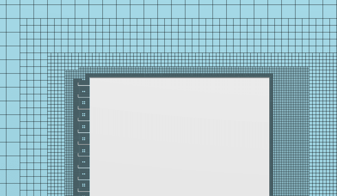
An automatic generation of many levels of refinement is offered by the LBM method, according to the dimensions of the modeled building with balconies. Six Refinement regions were generated by using this feature, and the final mesh had the following characteristics:
| Number of cells | Minimum cell length (mm) | Maximum cell length (mm) |
| 37 million | 0.73 | 23 |
The first parameter that was tested for correlation among the different CFD analysis models and experimental data is the mean surface pressure coefficient on the building with balconies that is defined as:
$$ C_p = {p – p_o \over \ 2 \times\ ρ\times \ U_{ref}^2}\tag{4}$$
where,
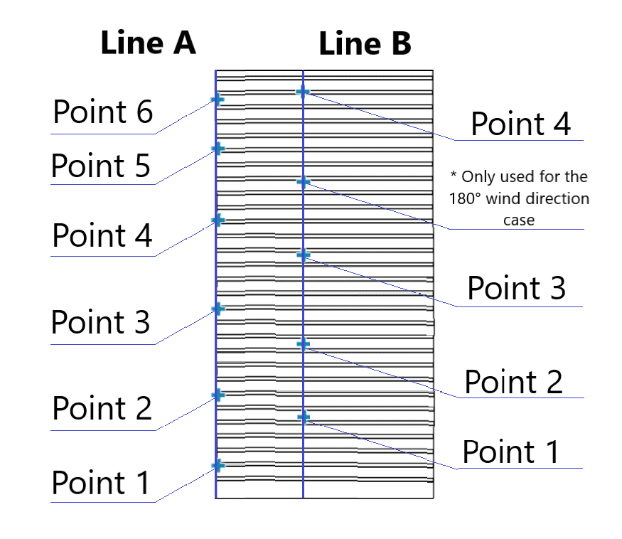
Two lines were used to inspect the correlation between the different solvers and the experimental data, Line A and Line B. 800 points were also used to extract the pressure values across each line.
Eleven points in total, placed on either Line A or Line B, were used as reference points for the evaluation.
Let’s breakdown the results for each wind direction:
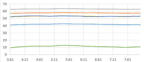
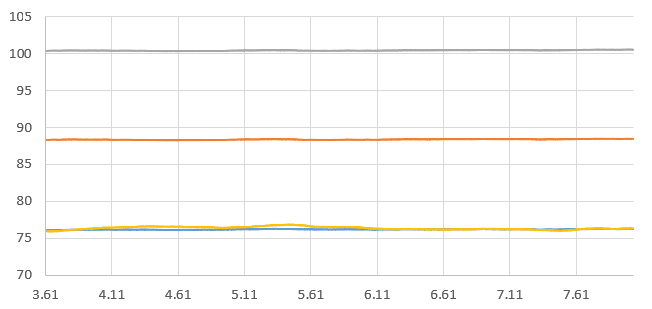
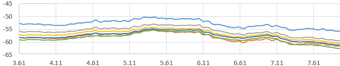
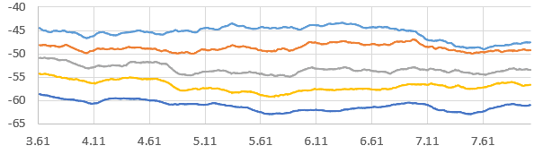
After the moving average of the results was calculated for a variety of fluid passes, 5 fluid passes were proved to be the best choice to be averaged and used as the outcome of the simulation. The moving average is an indicator used in technical analysis that helps smooth out price action by filtering out the “noise” from random short-term price fluctuations, identifying the trend direction. Especially, the arithmetic mean of a security over a number (n) of time periods, and it is defined as:
$$SMA = {ΔC_p \over \ n}\tag{5}$$
where:
A fluid pass is given as:
$$N = {L \over \ U_{ref}}\tag{6}$$
where:
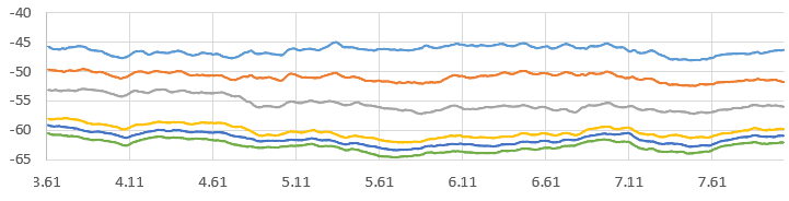
This is the moving average for the 5 reference points of Line A:
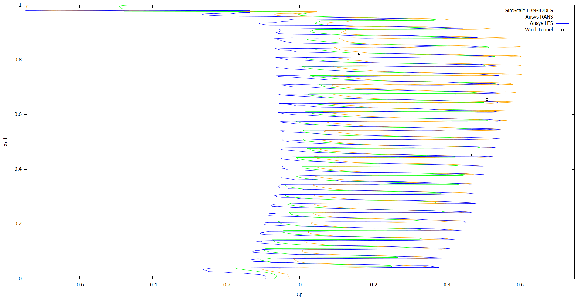
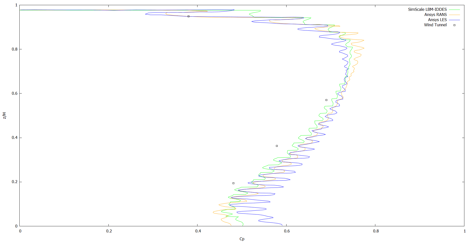
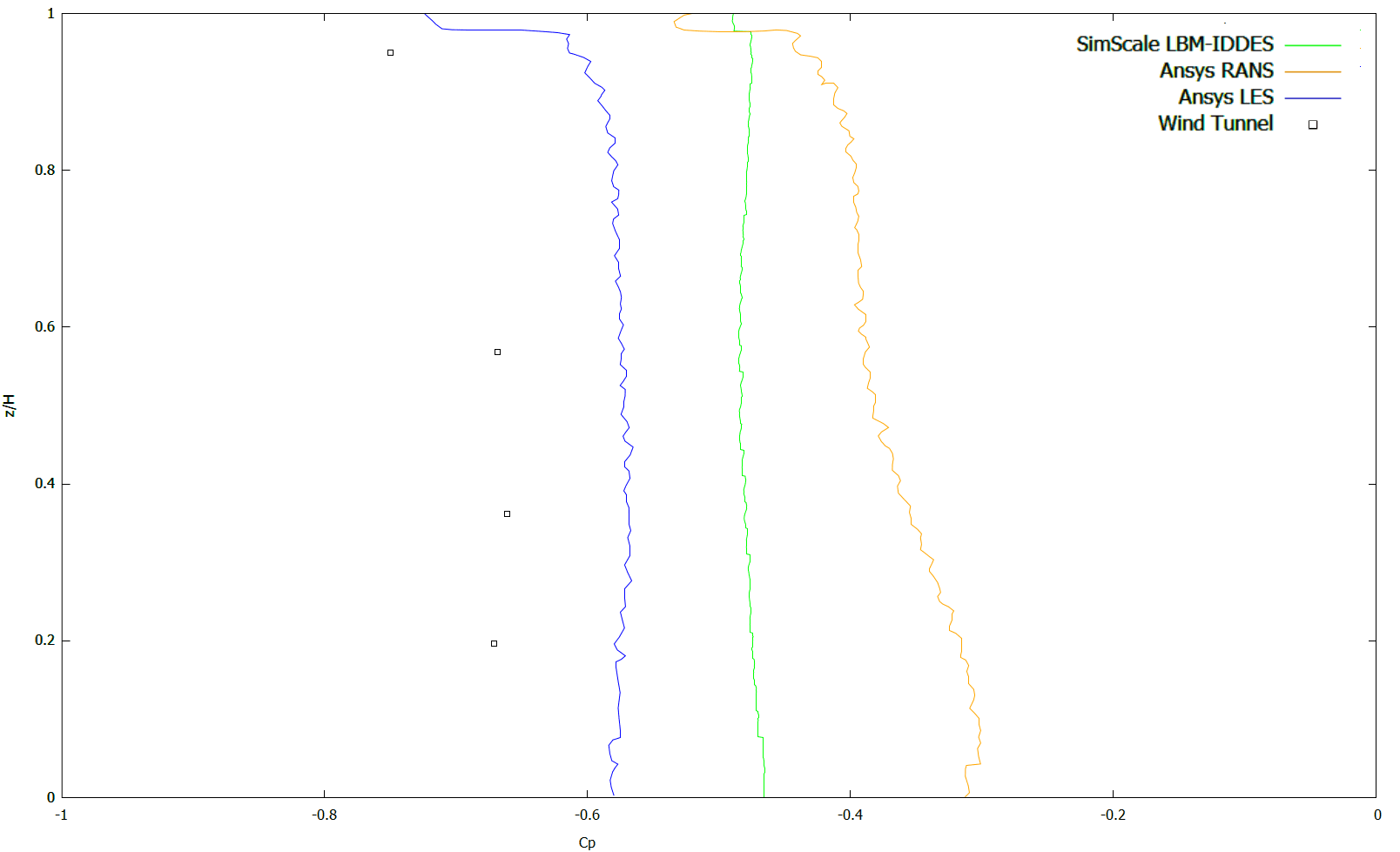
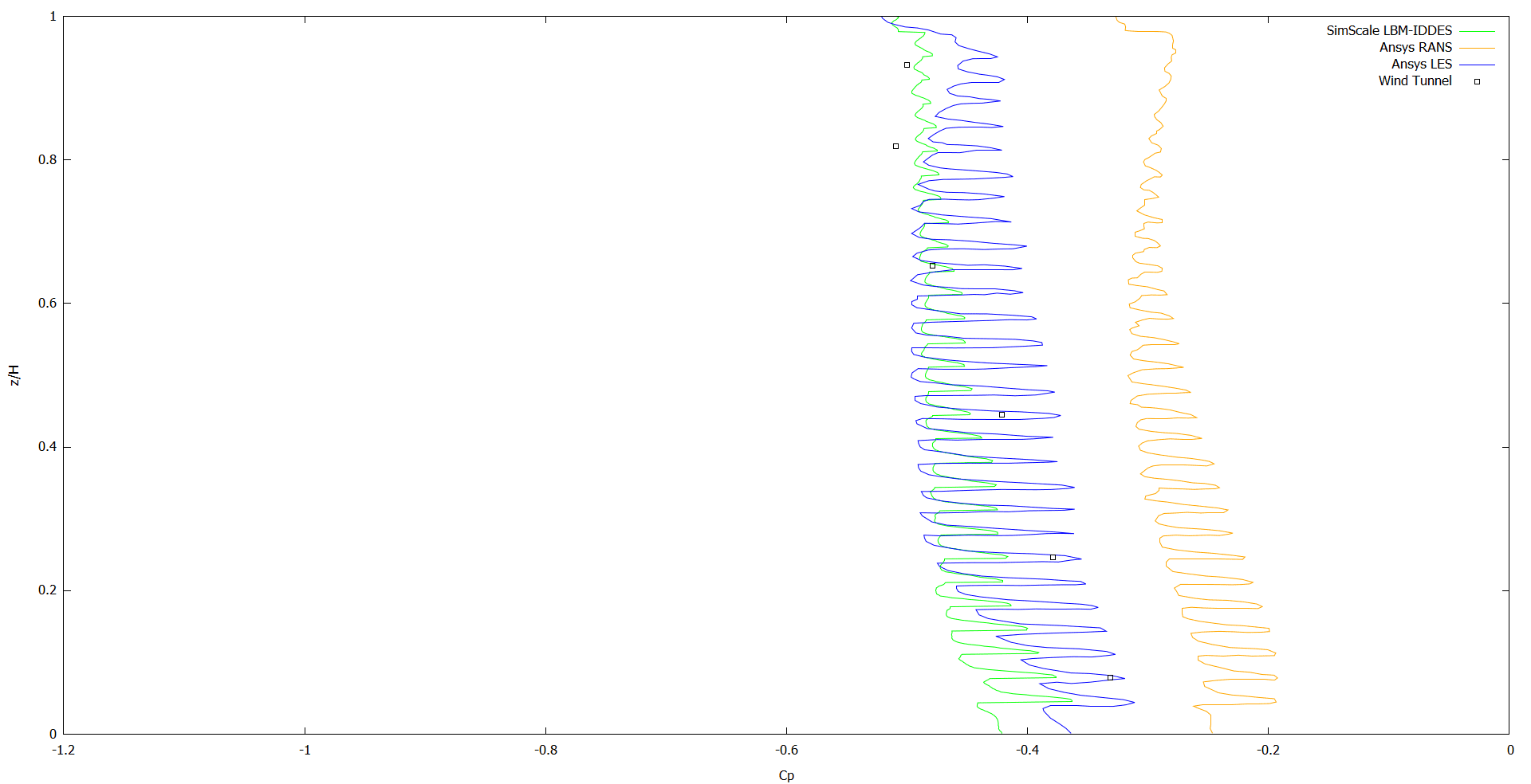
The Cp distribution across Line A can be seen below. The Ansys RANS, Ansys LES, SimScale IDDES and Experimental solutions are all included in the graph:
The same procedure is done for Line B too:
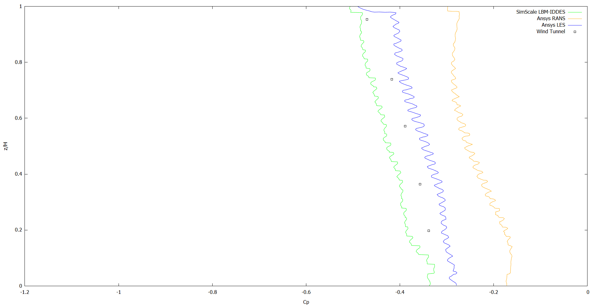
And the Cp distribution results across Line B are as follows:
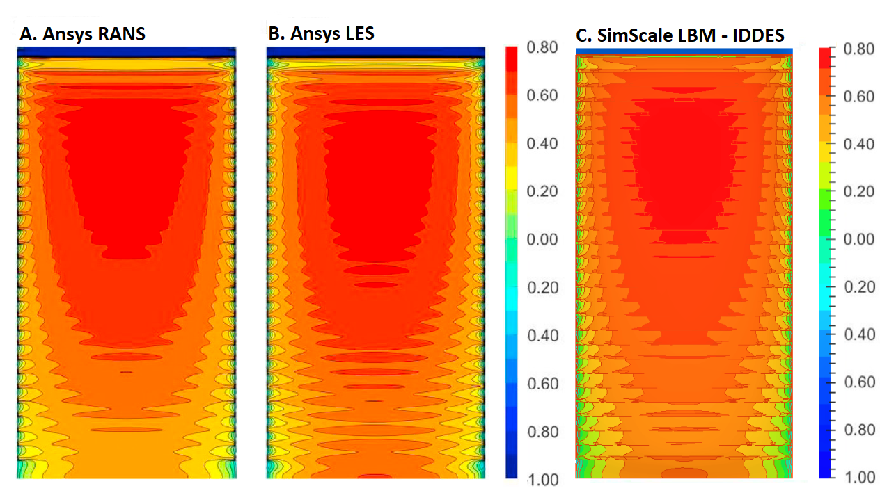
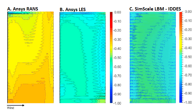
Also, a visualization of the Cp distribution results on the facade of the building with balconies was created, showing how close the CFD results are:
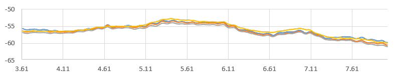
For the 90 degrees wind direction case, the moving average is not as stable as the 0 degrees case. This is the moving average for the 5 reference points of Line A:
Compared to averaging of a smaller amount of fluid passes , the 5 fluid passes was the most stable choice, and it was used for the Cp distribution graphs across Line A:
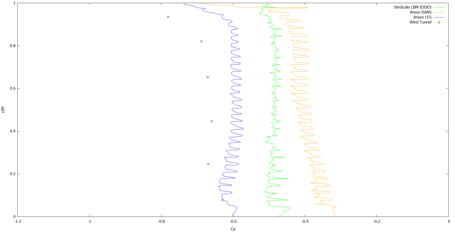
The same applies for Line B:
Cp distribution showing how the SimScale LBM-IDDES results are with respect to the Ansys LES and Ansys RANS across Line B:
However, the visualization of the Cp on the facade shows better resemblance in the Ansys LES case:
The respected moving average graph for the 180 degrees case is closer to the stability of the 0 degrees case for Line A:
The IDDES results are comparable to those of Ansys LES:
The same applies to the moving average of 5 fluid passes for Line B:
The IDDES results under predict the Cp, whereas the other two approaches seem to over predict it:
Finally, like the previous 2 cases, the visualization of the Cp on the facade showcases good agreement with the LES study, meaning a more reliable result than the Ansys RANS:

The velocity ratio, K, is an important parameter when it comes to assessing the pedestrian wind comfort. It is calculated as:
$$K = {U \over \ U_{ref}}\tag{7}$$
where:
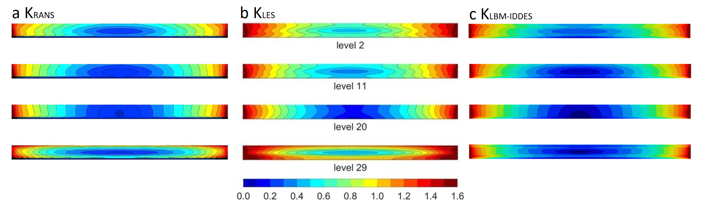
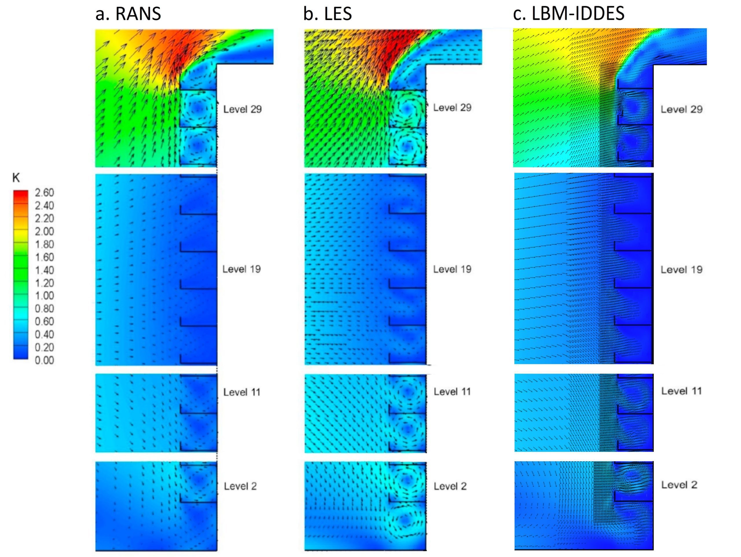
Below are some comparisons of the distribution for the K ratio across the balconies of Levels 2,11,20 and 29, at a height of 1.75 m (average person’s height) for the 0 degrees wind direction:
Also, the K distribution comparison across the vertical center line for the 0 degrees case was created:
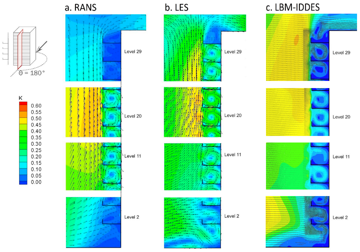
And a similar one for the 180 degrees wind direction case can be seen below:
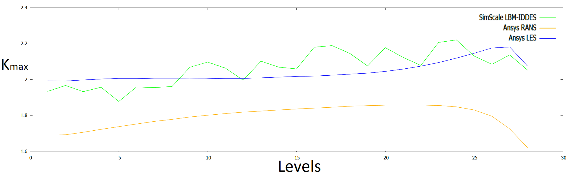
Finally, an evaluation of the maximum Velocity ratio, /(K_{max}/) was performed across the balconies for the 0 degrees wind direction.
$$K_{max} = (U_{max}/ times/ U_{ambient})\tag{8}$$
where:
A table that contains the metrics used for the deviation calculation is presented below:
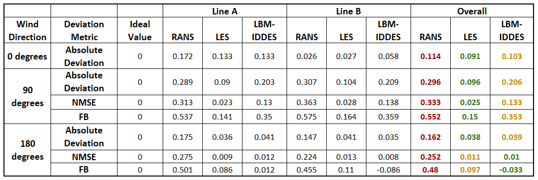
The metrics are:
$$NMSE = \frac{[(C_{p(WT)}-C_{p(CFD)})^2]}{[C_{p(WT)}][C_{p(CFD)}]}\tag{9}$$
$$FB = \frac{2([C_{p(WT)}]-[C_{p(CFD)}])^2}{[C_{p(WT)}]+[C_{p(CFD)}]}\tag{10}$$
A fluctuating inlet condition would help with the results. Also, not having an already converged flow field as an input affects convergence especially for the 90° wind direction.
All of the cases show better agreement with the experimental data than the RANS simulations. The 180° wind direction’s results are the closest to the LES results.
References
Last updated: January 2nd, 2024
We appreciate and value your feedback.
Sign up for SimScale
and start simulating now


