Validation Case: Pedestrian Wind Comfort: AIJ Case C
Introduction
With the increase in the number of high-rise buildings being constructed all around the world, proper planning of the close vicinity for comfort and safety becomes important. Computational fluid dynamics (CFD) is an apt solution for assessing these comfort and safety levels for pedestrian wind comfort (PWC) even before the buildings are erected, and also helps in faster design iterations. Pedestrian-level (micro-climate) condition is one of the first microclimatic issues to be considered in modern city planning and building design \(^1\).
Wind analysis results using CFD simulation are now seen as reliable sources of quantitative and qualitative data, and they are frequently used to make important design decisions. However, to have full confidence in those decisions, extensive verification and validation of the CFD results are necessary. For this, we will be validating against the experimental results provided by the Architectural Institute of Japan (AIJ), using AIJ Case C.
Architectural Institute of Japan (AIJ) Pedestrian Wind Comfort Experiments
The Architectural Institute of Japan (AIJ) is a Japanese professional organization for architects, building designers, and engineers. It was founded in 1886 and has gathered over 38,000 members since. It publishes several journals, technical standards for architectural design and construction, and research committee studies.
The wind analysis test case for this validation was taken from the “Guidebook for Practical Applications of CFD to Pedestrian Wind Environment around Buildings”\(^2\), published by AIJ in 2008, which sets the standards for cross-comparison between the results of CFD predictions, wind tunnel tests, and field measurements, and helps validate the accuracy of CFD codes for pedestrian wind comfort assessments.
AIJ Case C
Wind Analysis in an Urban Area
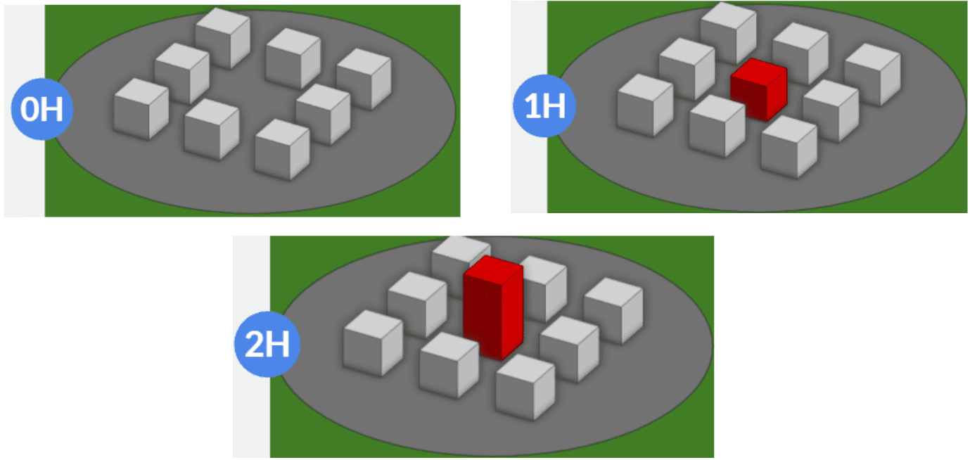
The purpose of this project is to use experimental results from the Architectural Institute of Japan\(^3\) to validate CFD results gained from SimScale using the LBM method provided by Numeric Systems GmbH. The case being validated is Case C in which AIJ provides experimental data for 9 cases, 0°, 22.5°, and 45° for 3 different geometries. The geometries represent a small block of buildings (see Figure 1) where there is
- No construction at its center
- Low rise building constructed at its center
- High rise building constructed at its center
The building model is a cuboid with a side length D of 0.2 \(m\). The reference velocity (UH) of the approaching flow at building height H (where H = D) was set to UH = 3.65 \(m/s\).
Geometry
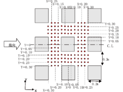
The CAD geometry was modeled based on the geometry data and specification that is available in the AIJ Case C datasheet \(^3\). The figure below shows the CAD model uploaded into SimScale with the main building highlighted in red, and an orange box representing the location of the measurements points which are shown in Figure 2.
where H represents the building height and is equal to D = 0.2 \(m\)
Simulation Setup
For this simulation, we used SimScale’s LBM solver, which is a different approach to traditional Finite Volume Methods. This solver is an implementation of Pacefish®, provided by Numeric Systems GmbH\(^4\), and has many advantages over the traditional approach, but the most relevant in this case are geometry robustness and solver speed. Since the solver runs on GPU architecture and scales very well, we can solve very large meshes in transient at a fraction of the time it would take traditional solvers to solve in steady-state.
A summary of the simulation setup is as follows:
- LBM solver
- K-omega SST DDES (LES in the far-field with K-omega SST wall modeling)
- Wind profile was defined using the Log law with a reference height of 0.2 \(m\), a reference velocity of 3.6\(m/s\) and an aerodynamic roughness value of 0.00045 \(m\).
- The ABL profiles were assigned on the upstream boundary while the downstream boundary was assigned a pressure outlet with a reference pressure of 0 \(Pa\).
- A no-slip wall without roughness was applied on the ground.
- A slip wall boundary condition was applied to all other faces of the virtual wind tunnel.
- A virtual wind tunnel was used that measured 8 \(m\) long x 4 \(m\) wide x 1.3 \(m\) tall.
Regarding the ABL profiles, Figure 3 below illustrates a comparison between both the velocity and turbulent kinetic energy (TKE) profiles generated by SimScale using the log law with the specifications mentioned above and the profiles from the AIJ Case C data. In Figure 3 the red dashed line represents the height of the building blocks which was 0.2 \(m\)
In Figure 3, “SimScale-Target ABL” refers to the ABL profile that is applied at the inlet, whereas “SimScale-Log Law ABL” represents the profile just before the city model, illustrated in Figure 4.
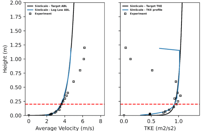
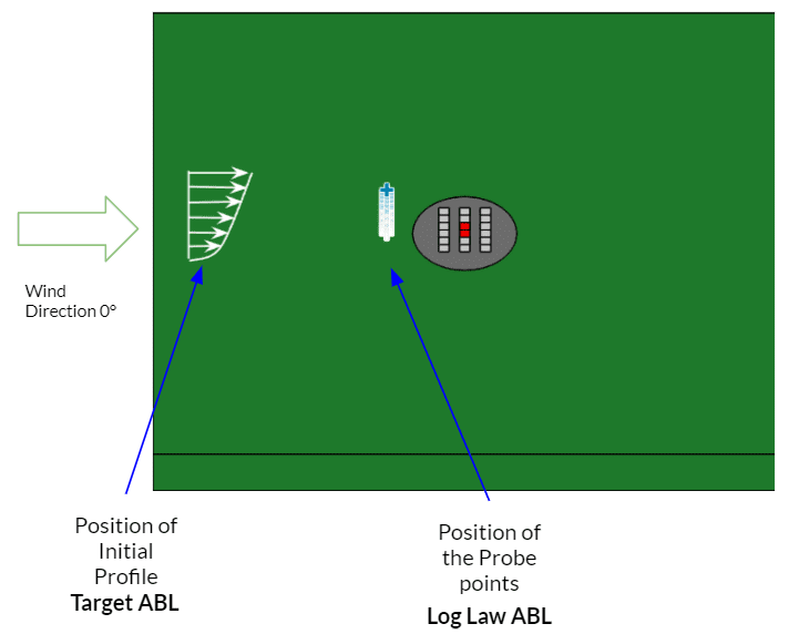
Maintaining a homogeneous ABL across the domain of the simulation plays a vital role in obtaining a reliable solution because it ensures that the wind conditions acting on the building of interest are the same as those intended by the modeller.
Meshing
For an incompressible LBM analysis, the meshing is based on the lattice Boltzmann method (LBM) and is quite different from the finite-volume based fluid dynamics analysis types in SimScale. Here a cartesian background mesh is generated, which is composed only of cube elements that are not necessarily aligned with the geometry of the buildings or the terrain.
To take into account the exact geometry, there exists a sub-grid model that accounts for the interfaces between the geometry and the fluid domains.
Turbulence Model
As mentioned before, the turbulence model K-omega SST DDES, which uses the highly regarded LES turbulence model in the far-field but uses the equally well-regarded wall model from the K-omega SST model, has proved itself particularly in the Aerospace Industry. The transition between the two models happens in the log-law region in the boundary layer. This means that we improve turbulence prediction by using LES, but also reduce its inherent cost by adding a robust wall model, reducing the mesh requirement at the wall.
Mesh information:
- Number of 3D cells: 82.5 Million
- Minimum cell size 0.0013 \(m\)
- Mesh decided upon based on a mesh convergence study. (see Figure 6)
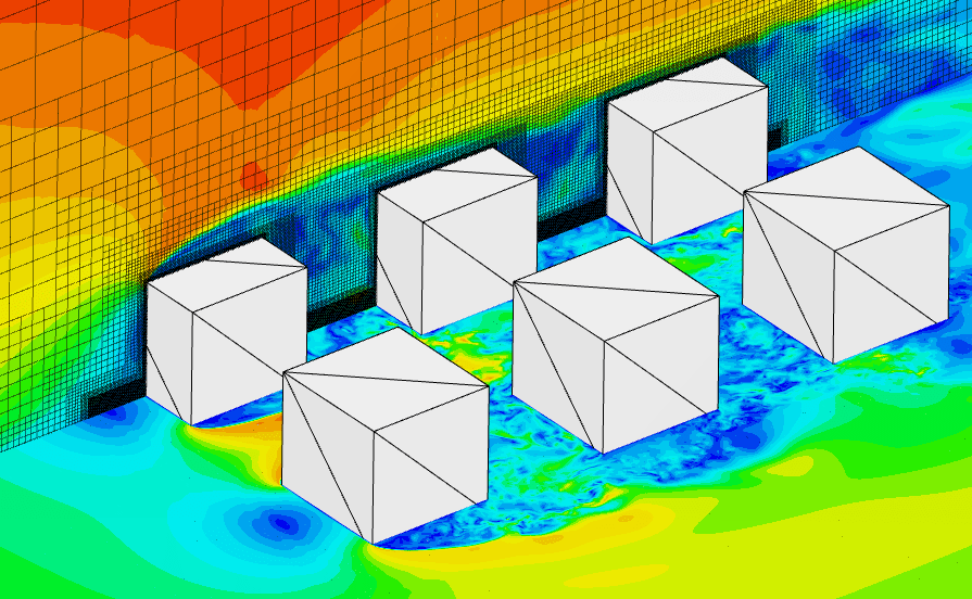
- Automatic Surface refinements with additional buffer cells on the wake region (see Figure 5)
- Region refinement (near floor) (see Figure 5)
Mesh Convergence Study:
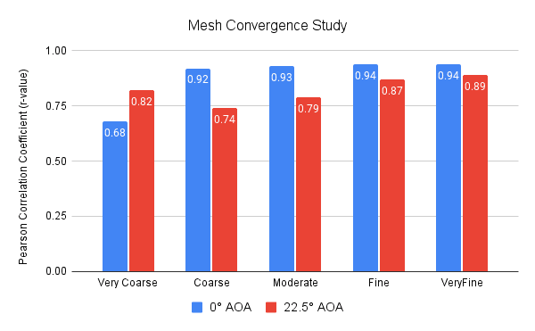
For the purpose of eliminating the dependency of the results on the mesh size, a mesh convergence study had been carried out. The results of this analysis are illustrated in Figure 6 using the Pearson correlation coefficient (r-value) between the velocity results obtained by SimScale and the experimental results from AIJ Case C.
The mesh convergence study consisted of the following:
- 5 different mesh sizes
- Two different wind directions namely:
- 0° and 22.5° AOA
- Performed on the CAD model which has the height of the center building as 1H.
Mesh Convergence Study Outcome:
- Multiple incoming wind configurations would translate to different flow structures.
- This means a mesh that converges for a certain setup might not be for a different one due to the changes in flow characteristics (i.e. due to different AOA)
- For a meaningful comparison, one surely has to keep the physics between the two setups exactly the same (i.e. BC’s)
- For the 0° wind (blue) it can be seen that the mesh converges around the coarse mesh. (Figure 6)
- For the 22.5° it can be assumed that the mesh converges around the fine mesh. (Figure 6)
- By combining these two information together and to provide a sufficient mixture between accuracy and computational efficiency → the Fine mesh had been chosen for further simulations.
Results
The results obtained from the simulation are validated with the wind-tunnel experimental data at the measuring points which are located at a height of 0.1D from the ground (where D is the dimension of the cuboid):
- The experimental data were measured by a thermistor anemometry with a sampling interval of 1 \(Hz\) and a sampling time of 30 \(s\).
The results from the simulation were averaged over the latter 50% of the simulation time to exclude results that are distorted by the time it takes for the simulation to stabilize.
To set the basis for the comparison, the velocity results that were obtained from the simulation at the measurement points (“validation points” in the simulation) were normalized by the inflow velocity at the measurement height of 0.1D. This is also stated clearly in the experimental datasheet of AIJ case-C \(^3\)
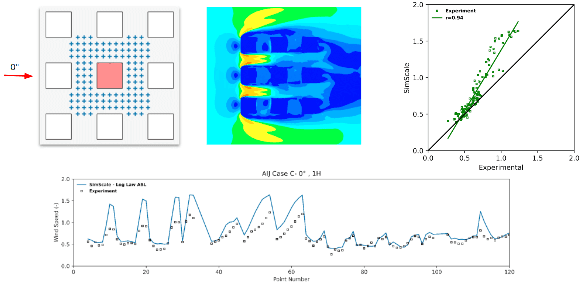
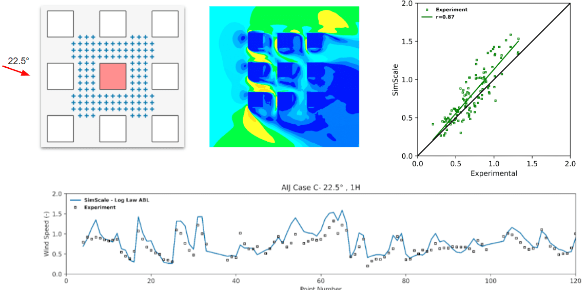
The results for the three analyzed wind directions are presented below in figures 7 through 12 by the means of 4 plots:
- Top left: Location of validation points
- Top middle: Color map of the velocity field
- Top right: Pearson correlation coefficient (r-value) plot between the experimental (x-axis) and SimScale results (y-axis)
- Bottom : Visual correlation comparison of the results at the location of the validation points
0° Wind Velocity Field
[0H, 1H, 2H]
22.5° Wind Velocity Field
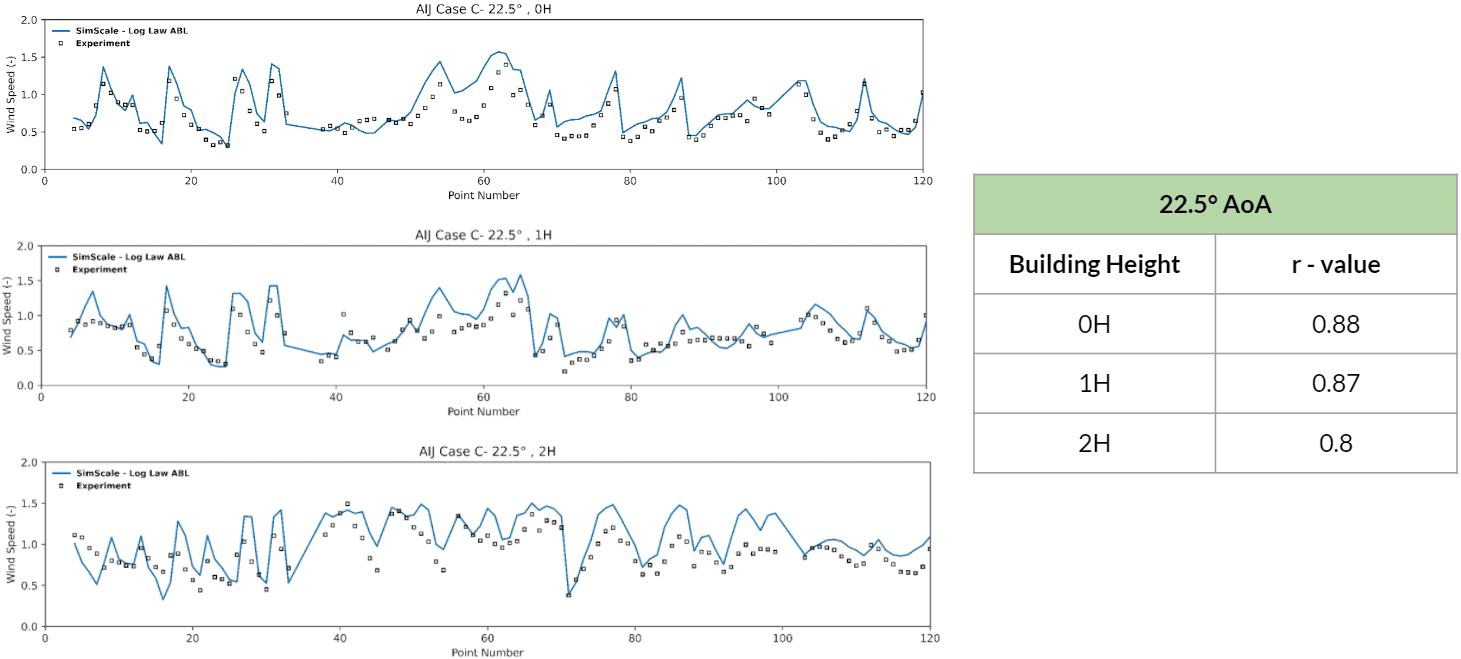
[0H, 1H, 2H]
45° Wind Velocity Field
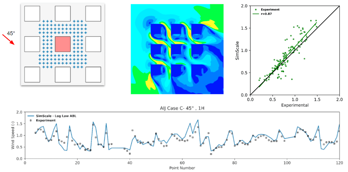
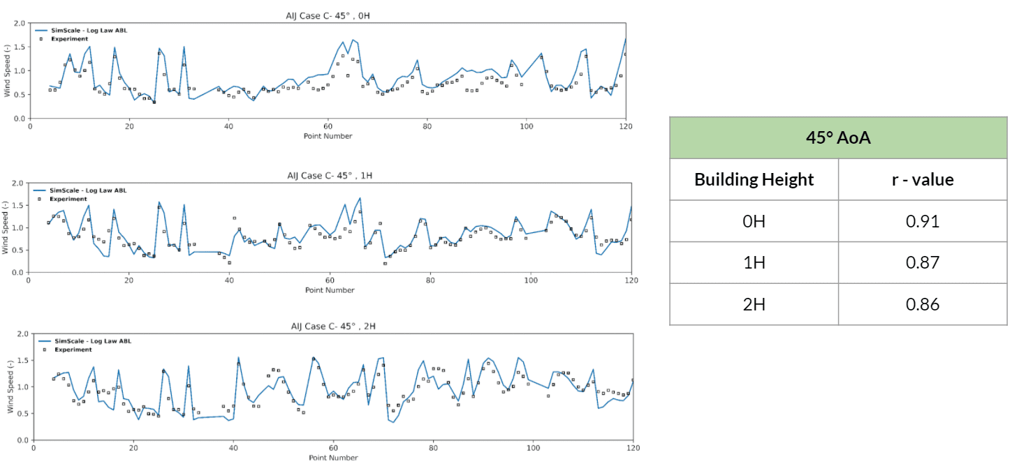
[0H, 1H, 2H]
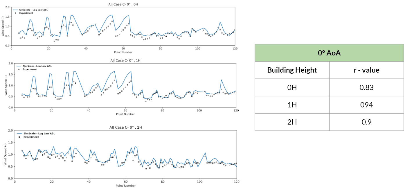
The results shown above are split into two parts for each of the simulated wind directions:
- Building height at 1H with r-value correlation plots
- Comparison between the results obtained for the varying height of the central building
By inspecting the results one can deduce that a very good corroboration exists between the SimScale and experimental results. The trend of the data from the wind tunnel experiments is very well approximated and the correlation coefficients attest to that by having values ranging from a minimum of 0.8 to a maximum of 0.94.
AIJ Case C: Conclusion
The purpose of this study was to validate the LBM method provided by Numeric Systems GmbH \(^4\) against the wind-tunnel experimental results of AIJ Case C. The results had shown a very good correlation to the wind tunnel data provided, where correlation coefficients ranging from 0.8 and up to 0.94 were obtained. Moreover, by inspecting the approximative trend of the SimScale results, one can visualize that it conforms to the pattern of the experimental data.
In general, both wind tunnel testing and CFD methods have their pros and cons and one cannot replace the other, especially when one understands that each is a different type of analysis which is suitable for different stages of a project and the type of information that you want to obtain from that particular study.
Usually, wind tunnel testing is mostly done for compliance testing and it is well known that it takes quite some time to set up the test and process the results and that it is quite expensive. All these factors make it quite difficult or infeasible to integrate it into an early design process. This leads to the fact where engineers derive value the most from CFD analysis because it allows them to obtain such a vital amount of information in the design process and can corroborate well to wind tunnel studies when validated.
Lastly, In terms of turnaround time, this validation quality mesh, consisting of 82.5 million cells, took just under 5 hours to solve, with an element resolution of 0.0013 \(m\), and cost around 20 GPU hours. In comparison to wind tunnel modeling this is a big advantage, but also against traditional finite volume methods, was much faster than the expected days of solve time for such a demanding mesh. The robustness of the solver also makes a large difference since there were no iterations to obtain numerical stability from the mesh, setup, and CAD quality, where experienced readers will know this is where they have traditionally spent the most amount of time.
References
- (104-106, 397-407) (2012) “Designing for pedestrian comfort in response to local climate ” Journal of Wind Engineering and Industrial Aerodynamics – Wu and Kriksic.
- (2006) “AIJ Guideline for Practical Applications of CFD to Wind Environment around Buildings” The Fourth International Symposium on Computational Wind Engineering – Akashi Mochida, Yoshihide Tominaga and Ryuichiro Yoshie. (Document: second to last)
- AIJ Case C wind tunnel results.
- Numeric Systems GmbH
Last updated: April 8th, 2022
Did this article solve your issue?
How can we do better?
We appreciate and value your feedback.


