Validation Case: 3D Dam Break

This validation case belongs to fluid dynamics and aims to validate the subsonic multiphase solver implemented in SimScale using a 3D dam break analysis. The case analyses a dam break with an overflow over a rectangular box. In detail, the following parameters are of interest:

• Gauge Pressure on rectangular block surface points \([Pa]\)
• Wave height at different points of the region of interest \([m]\)

The simulation results from SimScale were compared to the results presented by Kleefsman et al. in the study “3D dam break” \(^1\).

Geometry

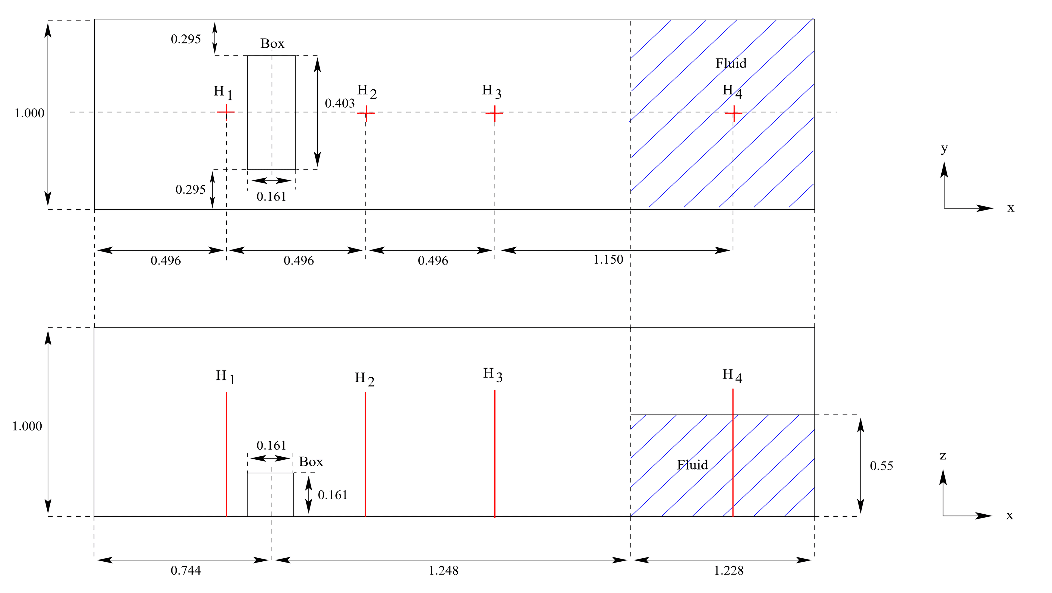
The dimensions of geometry are displayed in Figure 1. It shows the size of the simulation domain, the rectangular box, the initial water volume as well as the position of the height measurement points.

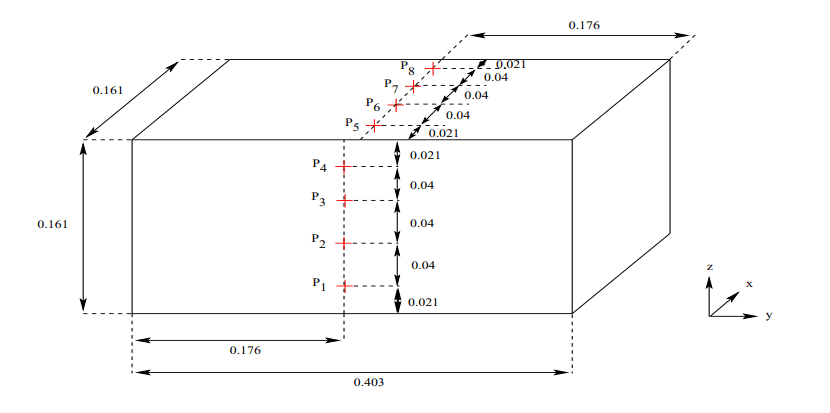
In order to measure the surface pressure on the rectangular box and the height of the water through the region of interest probe points were used. Figure 2 shows the positions of the measurement surfaces on the rectangular box.

Analysis Type and Mesh

Analysis Type: Transient, Subsonic-Multiphase, k-epsilon turbulence model

Mesh and Element Types:

The mesh was created with SimScale’s Subsonic meshing algorithm.

Mesh Sensitivity Analysis

The Subsonic meshing algorithm with hexahedral cells was used to generate the mesh. Multiple levels of fineness, from fineness levels 2 to 8, were used to perform the mesh sensitivity analysis. To correlate the data from different time steps of the surface pressure points on the rectangular box to the experimental data, a Pearson Correlation was performed. The results of the Pearson Correlation can be seen in Table 1 and Figure 3 below.

Mesh Level	Number of Cells	P1	P2	P3	P4	P5	P6	P7	P8	Average
2	116487	0.793	0.869	0.851	0.711	0.968	0.977	0.946	0.891	0.876
3	159799	0.848	0.884	0.919	0.767	0.804	0.795	0.638	0.583	0.780
4	230541	0.877	0.946	0.932	0.808	0.848	0.764	0.677	0.567	0.802
5	337444	0.880	0.933	0.946	0.855	0.839	0.888	0.822	0.700	0.858
6	504895	0.852	0.902	0.906	0.796	0.831	0.742	0.634	0.397	0.757
7	758092	0.894	0.928	0.921	0.806	0.788	0.755	0.676	0.469	0.780
8	1123321	0.889	0.918	0.888	0.789	0.869	0.808	0.702	0.566	0.804

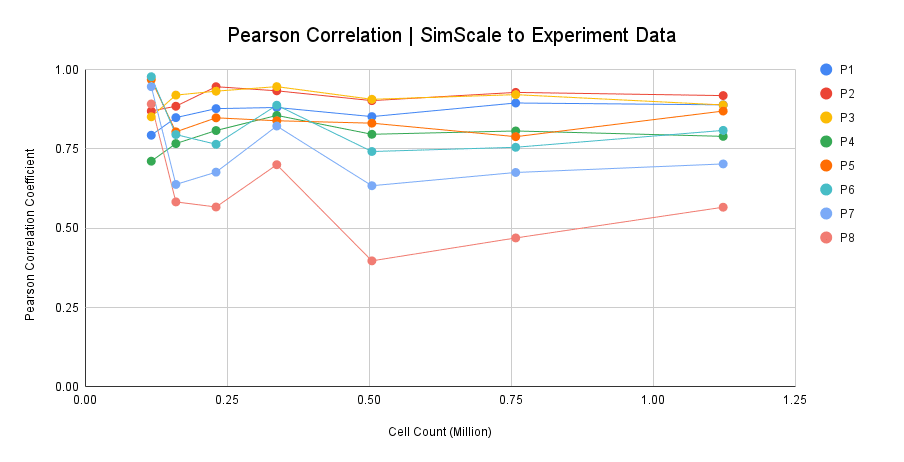
Mesh fineness levels 5 and 8 show a high correlation to the experimental data. Mesh fineness level 2 shows the best correlation with a very high correlation for every surface pressure point.

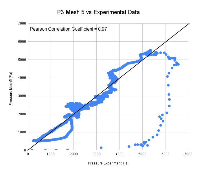
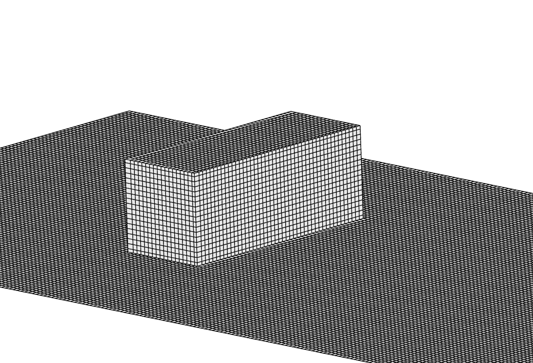
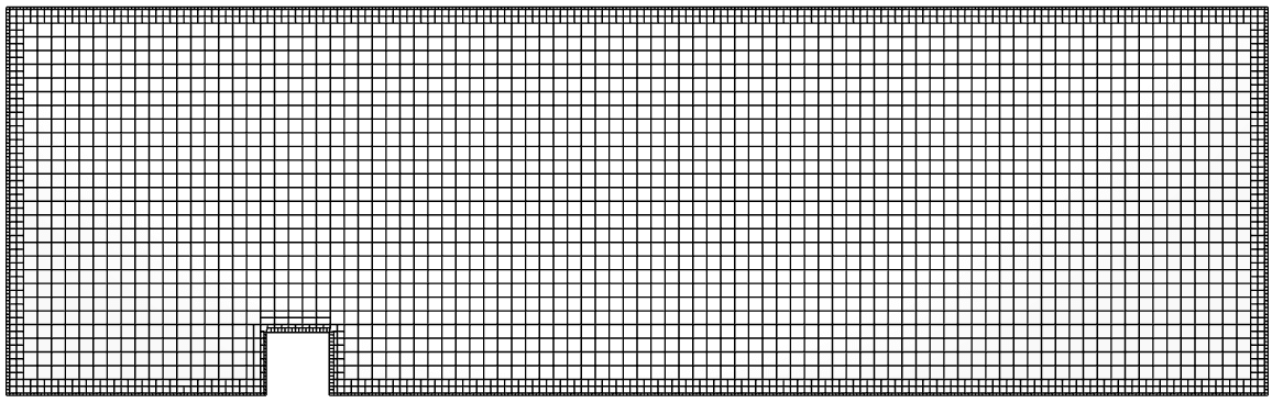
Figure 5 and Figure 6 display the surface mesh of fineness level 5 for the rectangular box and a cutting plane through the center of the region of interest respectively.

Simulation Setup

Materials

Fluids:

• Water
  • Kinematic viscosity \(\nu\): 9.338e-7 \(\frac{m^2}{s}\)
  • Density \(\rho\): 997.3 \(\frac{kg}{m^3}\)
  • Phase: 0
• Air
  • Kinematic viscosity \(\nu\): 1.5295e-5 \(\frac{m^2}{s}\)
  • Density \(\rho\): 1.196 \(\frac{kg}{m^3}\)
  • Phase: 1

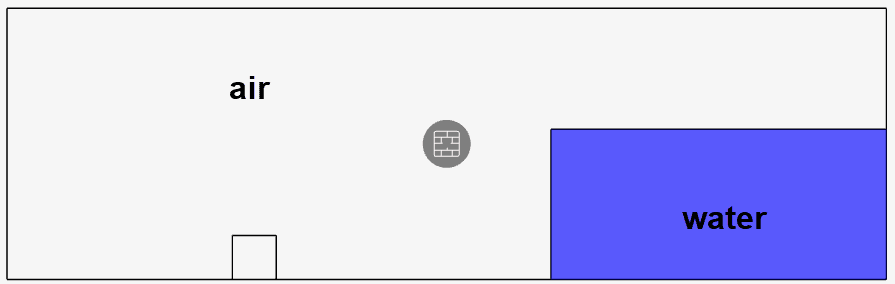
Initial Conditions

As initial conditions, the fluid volume for the different phases is defined. The initial regions for air and water can be observed in Figure 6:

Simulation Control

Run time and time steps

• Run Time: 5 \(s\)
• Time steps: 0.001 \(s\)

The simulation is transient and will be simulated to observe 5 seconds of real-time phenomenon. The computation will be carried out every 0.001 seconds.

Reference Solution

The solution is given for a time period of 5 seconds and compared to the results given by Kleefsman et al. \(^1)\. To calculate the height of the water at different positions the pressure at the bottom of the region of interest is measured and equation 1 is used to calculate the water height:

$$ Height_{Water} = \frac{Pressure} {g * \rho_{Water}} = \frac{Pressure} {9.81 * 997.3} \tag{1} $$

Result Comparison

Figure 7 shows the plots for the different surface pressure measurements points P1 to P8. Especially the frontal face points P1 – P4 show a good qualitative correlation to the experimental reference. Where P5 – P8 also show a good qualitative correlation of the data after 2.5 seconds.

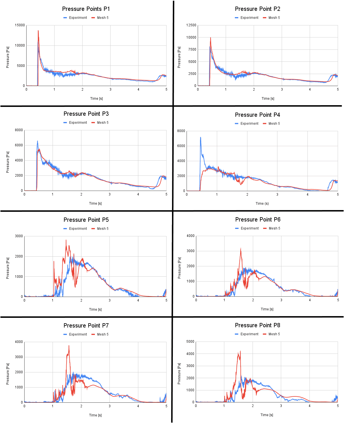
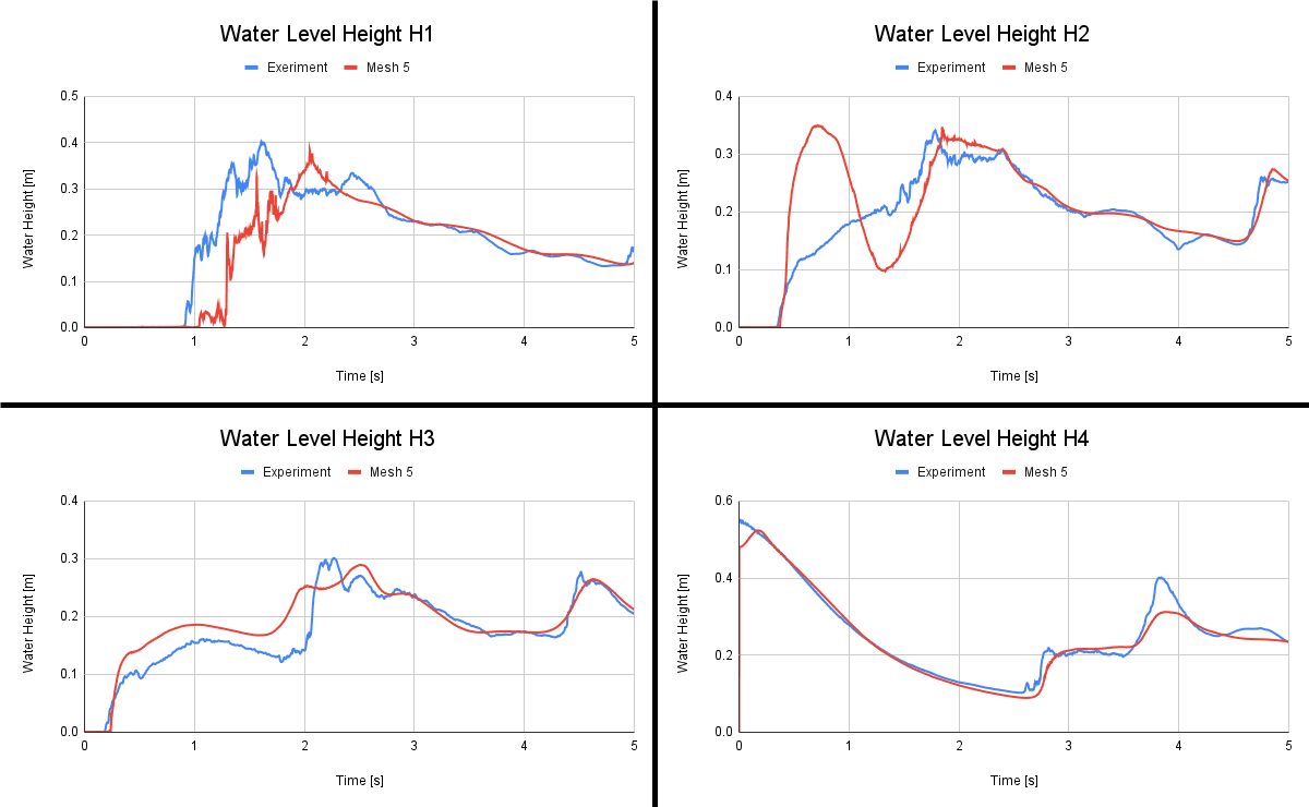
Figure 8 shows the height measurement data for the four bottom surface measurement points. All plots show a similar behavior as the experimental data. For plots H1 – H3, the time needed by the fluid to reach this measurement point from the initial condition matches quite well with the experimental data. In addition, height point H4 shows a good qualitative correlation to the experimental data, whereas H1 – H3 shows a good correlation for the period after 2 seconds.

In Animation 1 a comparison between the recorded experiment from Kleefsman et al. and a recorded animation from the SimScale results can be seen. The SimScale animation displays an Iso-volume of the water phase fraction with a volume phase fraction range from 0.3 – 1.

Last updated: January 9th, 2024