Thermal Management Tutorial: CHT Analysis of a Raspberry Pi Using IBM

This advanced thermal management tutorial describes the setup and analysis of the cooling of a Raspberry Pi box in an ambient environment. The scenario consists of an enclosure with several components cooled by a fan. The simulation utilizes the Immersed Boundary Method (IBM), which is resilient to complex geometrical details and does not require extensive CAD simplification.

The modern Raspberry Pi packs a significant amount of processing power into a small footprint. This density leads to rapid heat buildup. Without proper cooling, the Raspberry Pi faces two primary risks: Thermal Throttling and reduced Hardware Longevity.

Therefore, thermal management is crucial for system reliability and preventing failure.

In this context, CFD helps visualize and optimize airflow within the cramped constraints of a Raspberry Pi enclosure. Instead of relying on guesswork, CFD allows designers to eliminate “dead zones” (stagnant pockets of hot air), optimize heatsink geometry, and refine passive or active cooling strategies.

This tutorial demonstrates how to:

• Select suitable boundary conditions for thermal management and electronics cooling
• Assign materials for different components
• Define a fan region
• Use the IBM solver

The tutorial follows the SimScale workflow:

Set up the simulation

1. Create the mesh
2. Run the simulation and analyze the results

1. Select the CAD Model and the Analysis Type

Import the tutorial project into the Workbench by clicking the button below:

Clicking this link opens the following view:

1.1 Saved Selections for the Silicon Components

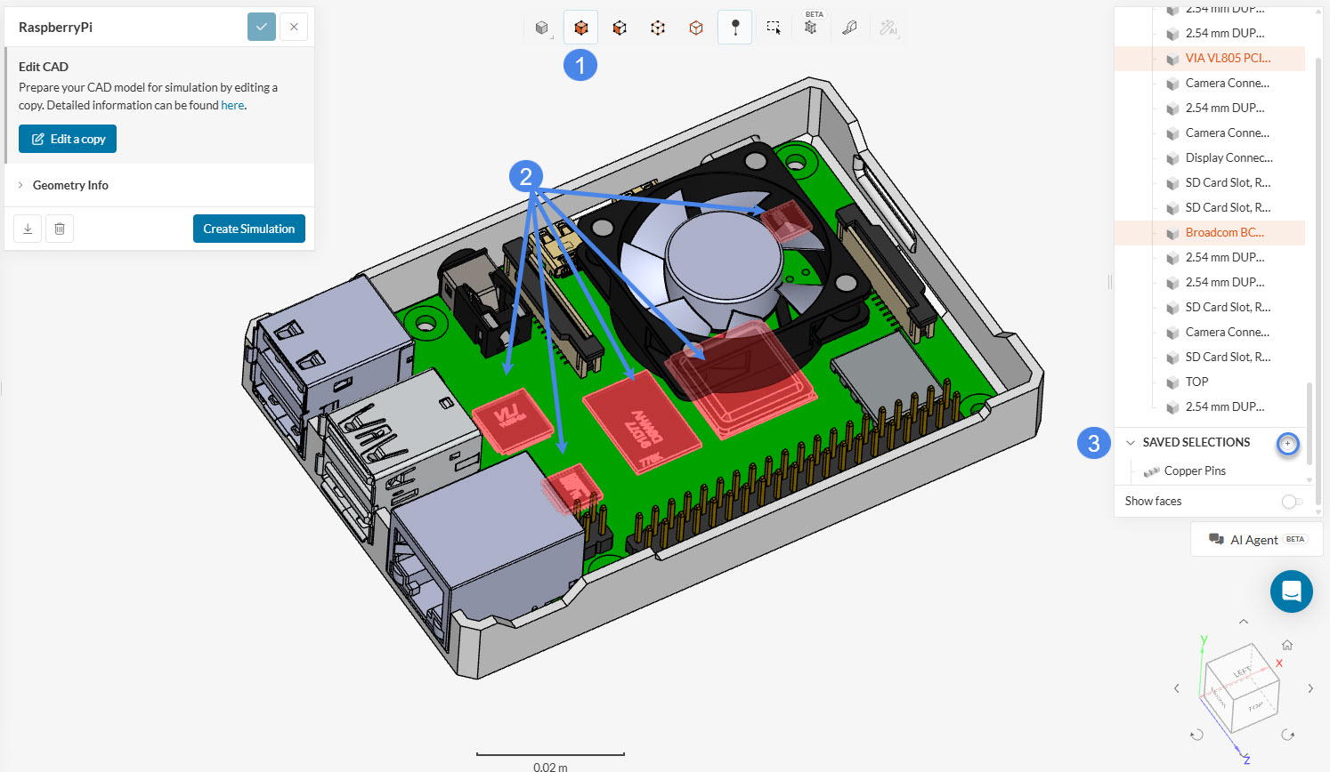
To streamline the workflow, this tutorial includes Saved Selections that allow for the rapid assignment of materials to specific regions. While pre-configured geometry can be used to skip this step, creating custom sets is a useful skill. Switch to volume selection mode, expand the geometry parts list, and select the components. Once selected, click the ‘+’ icon next to Saved Selections and name the set ‘Silicon’.

2. Simulation Setup

2.1 Create a Simulation

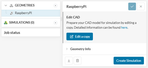
Once all saved selections are ready, select the ‘RaspberryPi’ geometry and click the ‘Create Simulation’ button as shown below:

The analysis selection widget will appear:

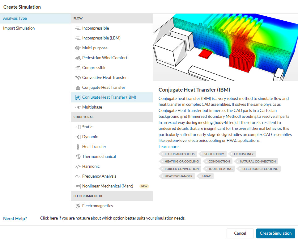
The analysis type widget lists all available options in SimScale. For this thermal management simulation, select ‘Conjugate Heat Transfer (IBM)’ and click ‘Create Simulation’ to confirm.

2.2 Global Settings

Upon creating a CHT (IBM) simulation, the simulation tree on the left panel displays Conjugate heat transfer (IBM), as shown below:

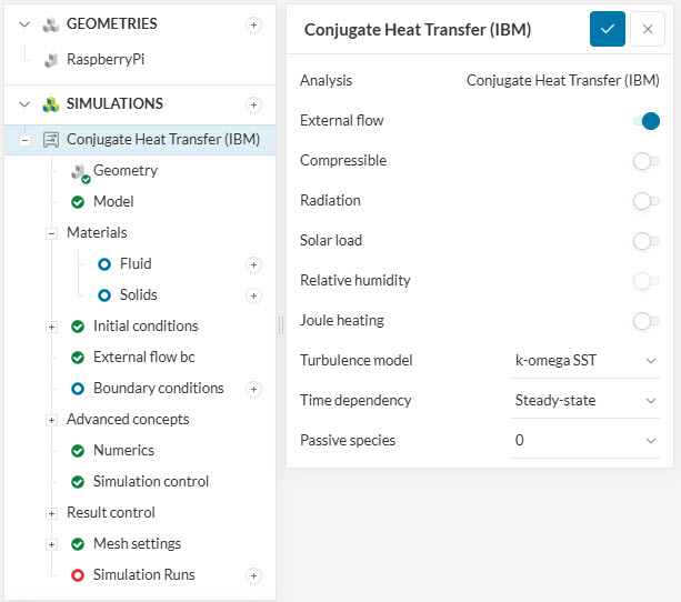
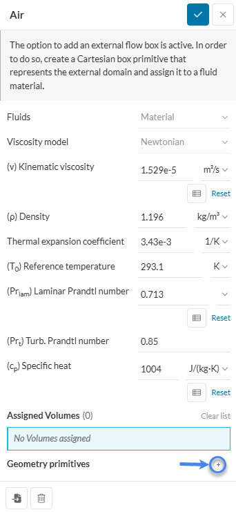
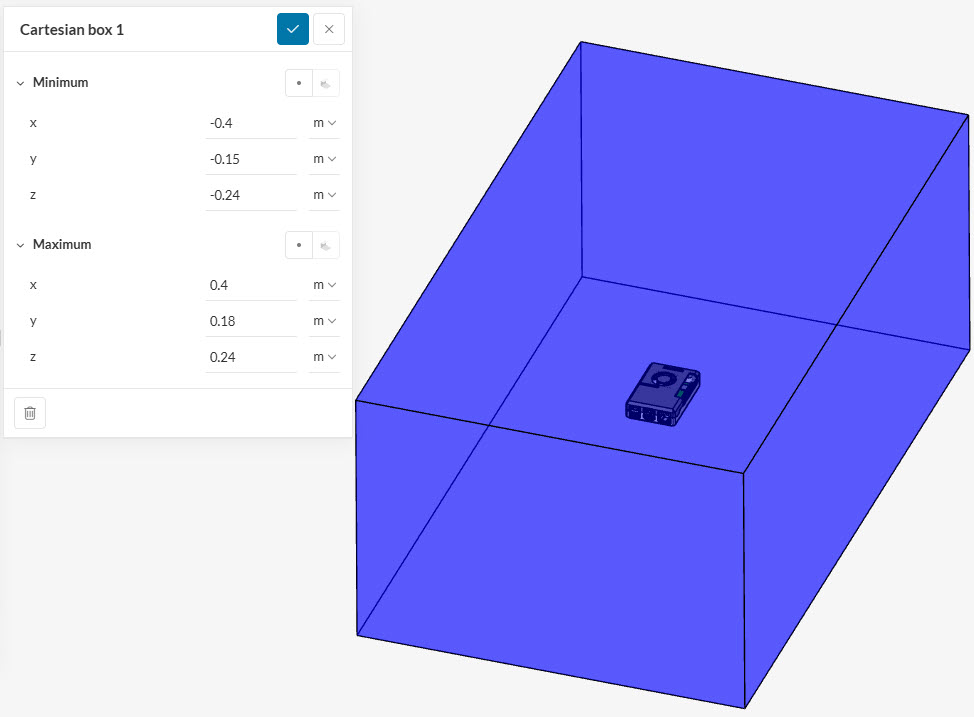
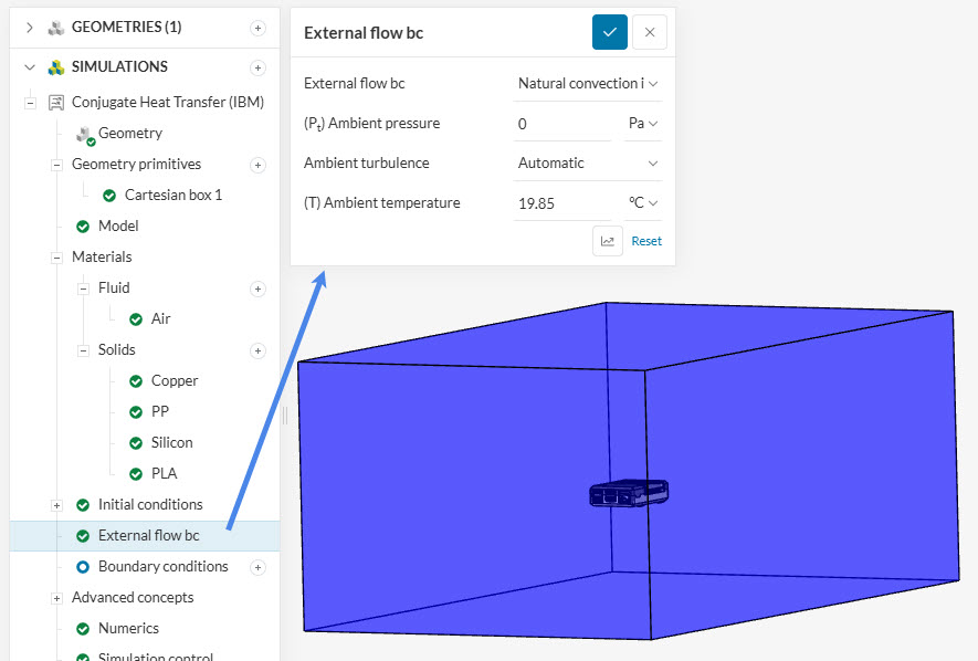
Access the global simulation settings and toggle on the ‘External flow’ option. The IBM solver allows for the generation of a flow region using a geometry primitive during setup. Alternatively, an internal flow volume can be prepared and imported manually without enabling automatic external flow generation.

Radiation remains toggled off for this tutorial.

2.3 Geometry

The Geometry tab can be skipped as the correct geometry is already in use.

2.4 Model

The Model tab defines gravity magnitude and direction based on the global coordinate system:

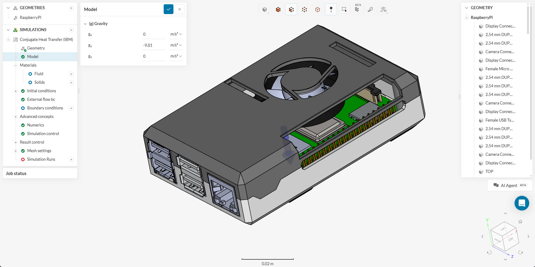
In this tutorial, gravity is set to ‘-9.81’ \(m/s^2\) in the ‘Y’ direction. Gravity definition is particularly important for natural convection scenarios.

2.5 Materials

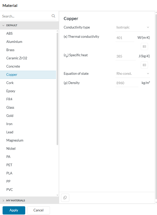
Material assignment for the various electronic box components follows. The table below summarizes these assignments.

Material	Saved Selections
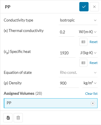
PP	PP
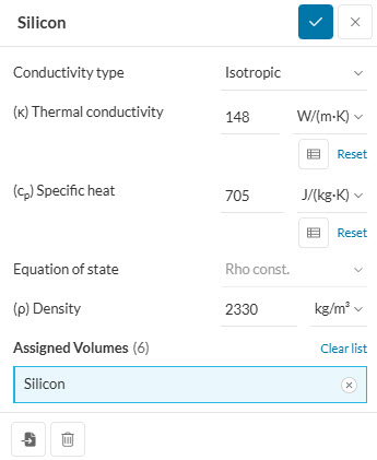
Silicon	Silicon
Copper	Copper Pins
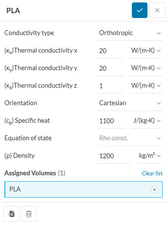
PLA	PLA Board

Most materials use default settings, though custom materials can be defined in SimScale.

1. Fluid Materials (Air)

To define a new fluid, click the ‘+’ next to Fluids to open the library:

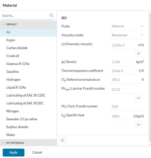
Select ‘Air’ and click ‘Apply’. A prompt will then indicate the need for a geometry primitive to represent the external flow region.

Click the ‘+’ icon and define the coordinates for a ‘Cartesian Box’. Once created, assign it as the ‘Air’ material.

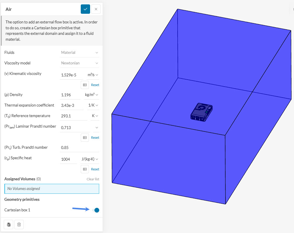
Hiding assigned parts by clicking the eye icon in the Saved Selections list facilitates visualization of subsequent steps.

2. Solid Materials (Copper)

Select the ‘Copper’ material from the library for the pins. Click the ‘+’ button next to Solids to view the list:

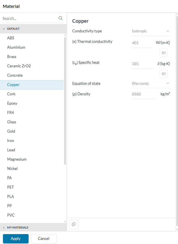
Select ‘Copper’ and click ‘Apply’. Assign this to the ‘Copper pins’ using the Saved Selections or direct interface selection.

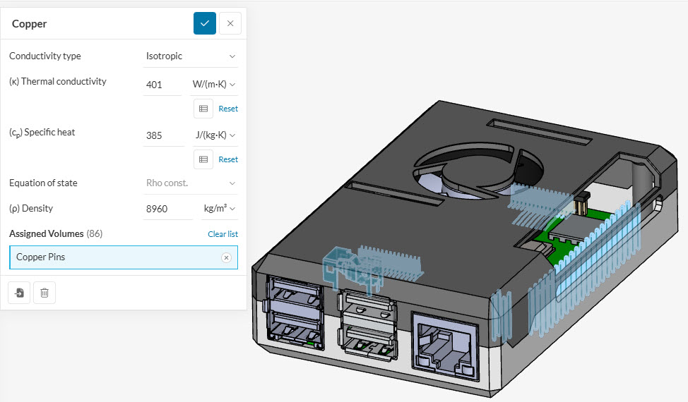
The Copper pins volume can be hidden after assignment to simplify the workflow.

3. Solid Materials (PP / Silicon / PLA)

Following Table 1, assign the remaining solid materials. Repeat the previous steps and select the corresponding materials from the library.

PP

Silicon

PLA (Polylactic Acid)

PCBs often exhibit anisotropic thermal conductivity. To reflect this, change the ‘Conductivity Type’ to Orthotropic. This enables unique thermal conductivity values for each axis. Specific heat and density values should also be updated as shown:

2.6 External flow bc

With ‘External Flow’ enabled (Fig. 6), SimScale automatically applies ‘Natural Convection inlet/outlet’ boundary conditions to all fluid domain faces. This permits flow in and out of the domain while allowing for ambient temperature and pressure adjustments. No further environment boundary conditions are needed.

2.7 Advanced Concepts

2.7.1 Defining Power Sources

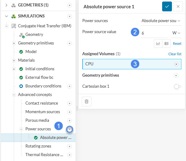
Heat dissipation from electronic components can be defined using power sources. This tutorial assigns power sources to the main CPU and smaller chips. The CPU power consumption is defined as \(6\) \(W\), representing a worst-case scenario for overclocking.

The following table details the power source assignments.

Saved Selections	Power Source \([W]\)
CPU	6
Chips	0.5

The individual power source configurations are shown below:

a. CPU

1. Under Advanced concepts, click the ‘+’ next to Power sources and select ‘Absolute power source’.
2. Define the heat dissipation as ‘6’ \(W\) for the CPU.
3. Assign the source to the ‘CPU’ selection.

Follow the same workflow for the other heat source:

b. Chips

Note that when assigning an absolute power source to multiple volumes, the specified value is applied to each volume individually.

2.7.2 Defining a Momentum Source

The model includes fan geometry to facilitate forced convection. SimScale provides two primary methods for fan modeling:

• Momentum Source: This method applies a mathematical force to accelerate fluid axially without physically rotating blades. It supports fixed velocity or fan curves.
• Rotating Region: This high-fidelity approach involves physical blade rotation. Velocity is generated by blade kinematics, providing realistic results at a higher computational cost.

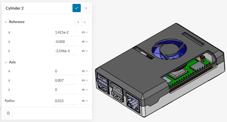
For this tutorial, a ‘Momentum Source’ with fixed velocity is used. Add a ‘Momentum Source’ and select ‘Average Velocity’. Set the velocity to ‘-5’ \(m/s\), ensuring alignment with the fan intake. Create a ‘Cylinder’ geometry primitive to define the volume for this source.

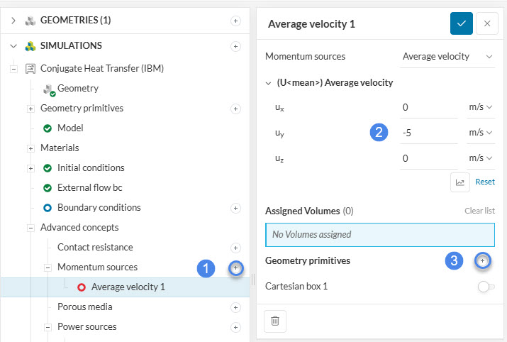
Align the cylinder with the fan center, encapsulating the blades. Use the coordinates provided in Table 3.

Reference	Value \(m\)
X	0.0142
Y	-0.0080
Z	-0.0036

2.10 Simulation Control

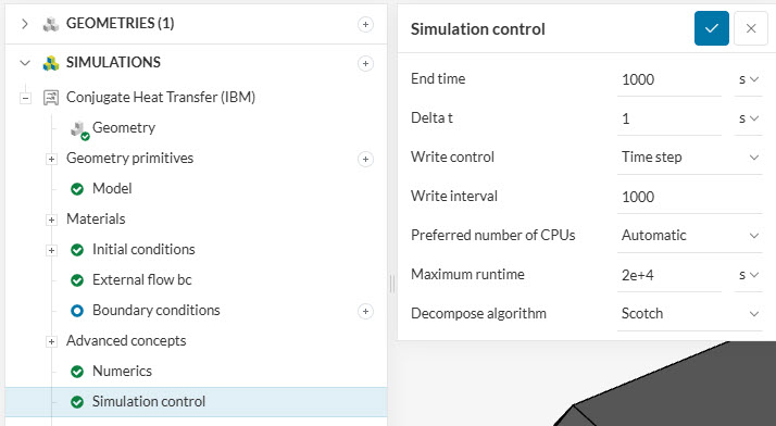
Default settings for Numerics are generally suitable. Simulation Control defines global parameters; these are kept at default values.

2.11 Result Control

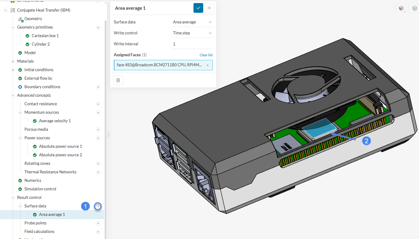
Velocity, pressure, density, and temperature are saved for every cell by default. Result control items can track specific points or surfaces throughout the calculation. This tutorial uses two items to analyze airflow.

2.11.1 CPU Temperature

To evaluate CPU temperature, create an area average on the CPU top face. This tracks physical data for the surface during every iteration. Follow the steps in Figure 23:

1. Click the ‘+’ next to Surface data under Result control and choose ‘Area average’.
2. Assign it to the CPU top face.

2.11.2 Probe point

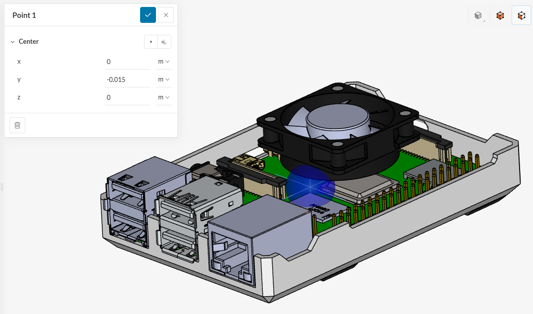
Probe points act like thermocouples, monitoring local variable values within the domain. They are useful for evaluating internal and external regions.

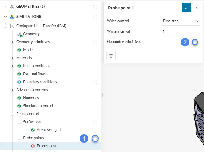
Create a ‘Probe Point’ with a ‘Y’ coordinate of ‘-0.015’ \(m\) to place it near the model center. Hiding the enclosure top face facilitates verification of the location.

Result controls are recommended for tracking key parameters like flow rates, pressure drops, and critical surface temperatures.

3. Mesh

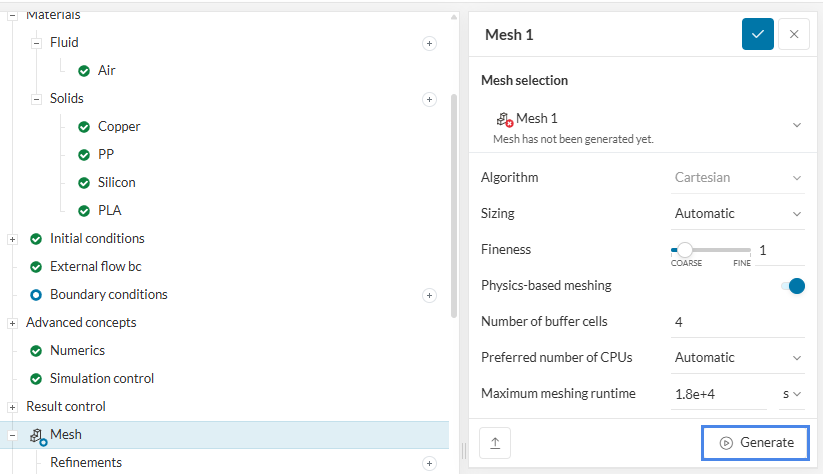
IBM simulations utilize Cartesian meshes that immerse geometry into a global grid. Advantages of IBM include:

• Versatility: Handles complex CAD with flexible sizing.
• Robustness: Automatically manages small geometric errors.
• Stability: Uses high-quality hexahedral cells.
• Physics-Driven: Focuses refinement on flow characteristics.

Set ‘Automatic Mesh Fineness’ to ‘1’ for a fast calculation. Click the Generate button to create the mesh, or you can start the run, and the mesh will be generated during the simulation.

4. Start the Simulation

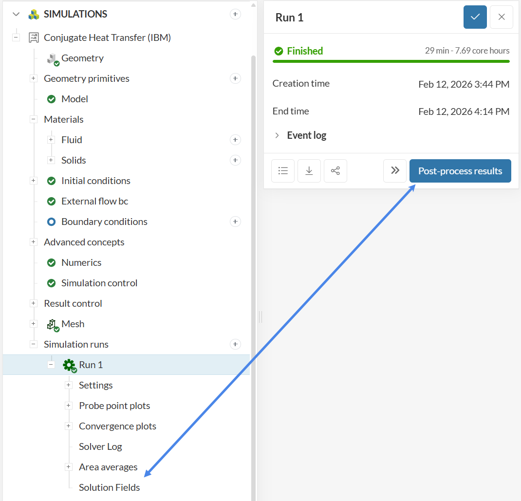
Click the ‘+’ icon next to Simulation Runs to begin the analysis. The mesh is generated and the solver starts automatically.

Intermediate results can be inspected in the post-processor in real-time while the calculation is ongoing.

5. Post-Processing

Once complete, access the ‘Convergence plot’ and ‘Solution fields’ from the simulation tree as shown below:

5.1 Convergence and CPU Temperature

In steady-state analysis, results should converge to a point where flow characteristics remain constant. This behavior can be monitored during and after the run.

a. Convergence Plot

Residuals represent the difference between calculated solutions for each mesh cell. Lower residuals indicate more stable solutions. Figure 28 shows the convergence plot for the solution variables.

1. Select the completed simulation run.
2. Open ‘Convergence plots’ and ‘Residuals’.

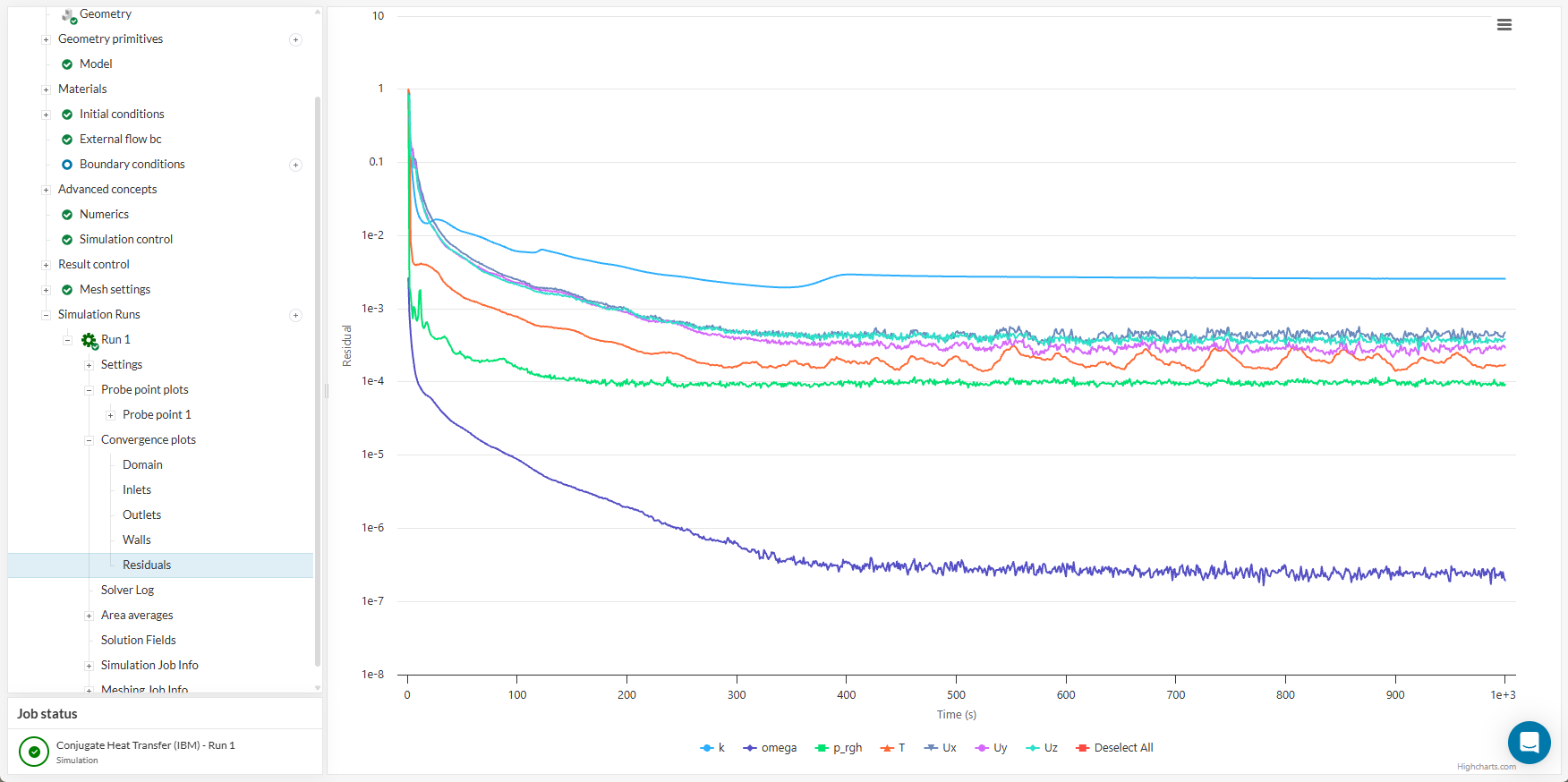
In this tutorial, all graphs remain below ‘1e-2’, with some dropping below ‘1e-3’, indicating good convergence.

b. Result Control

CPU temperature is a reliable parameter for evaluating design performance. The plot below shows the face temperature results.

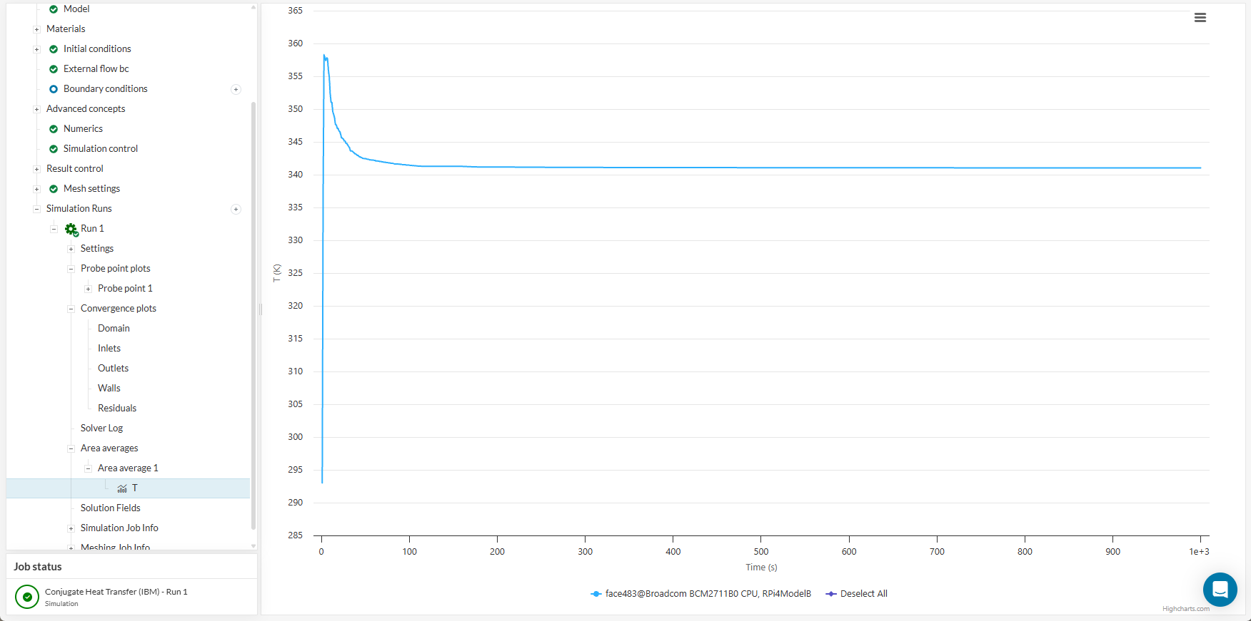
The temperature approaches a horizontal line, confirming a steady-state result. The average temperature of 340.03 \(K\) (40.88 \(°C\)) represents the cooling efficacy of the active fan. For comparison, the case can be simulated without the momentum source to evaluate passive cooling performance.

How to Check Convergence of a CFD Simulation?

5.2 Surface Visualization

Visualizing temperatures and the flow field can be done via ‘Solution Fields’ or ‘Post-process results’.

5.2.1 Temperature

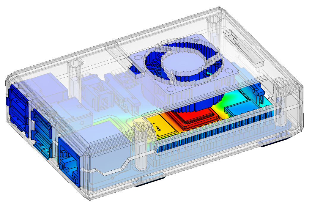
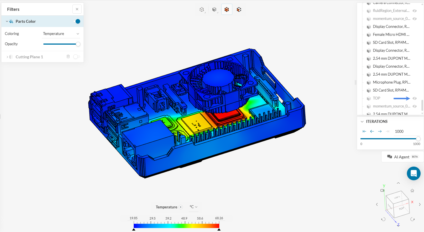
Initially, inspect the entire domain temperature. Hide the cutting plane and select ‘Temperature’ for Coloring. Right-click the screen and choose ‘Show all’ solids. Hide the external fluid domain and momentum source. Change the units to \(°C\). Right-click the legend bar and select ‘Use continuous scale’ for smoother visualization.

1. Toggle off the cutting plane visibility.
2. Set units to ‘\(°C\)’.
3. Select ‘Use continuous scale’ on the temperature legend.

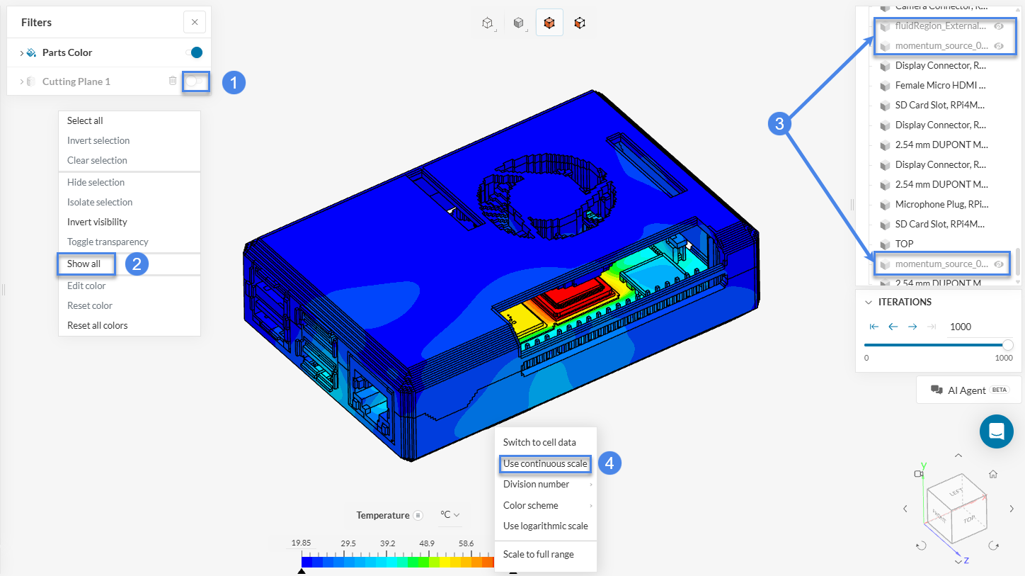
Hide the ‘TOP’ enclosure part in the geometry tree to view internal chips. Alternatively, select the part in the viewer and right-click to hide it.

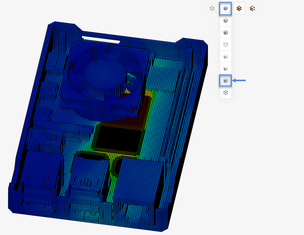
To inspect IBM mesh resolution, select the ‘Change render mode’ icon and switch to ‘Surfaces with mesh’. The IBM approach generates a “stair-stepped” grid that prioritizes primary domain features. While this mesh is coarse, surface refinements can be used for higher resolution of geometric details.

Hiding the fan region solids reveals how temperature affects the PCB.

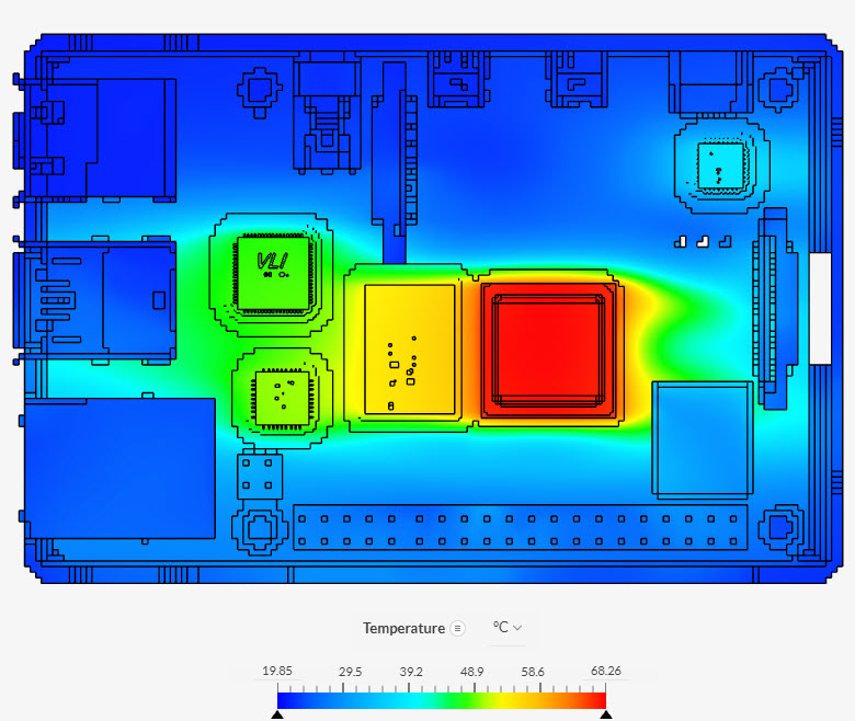
Results identify the CPU as the peak temperature region. CHT effects are clearly captured, showing thermal conduction through solids and interaction with the surrounding fluid.

5.3 Cutting Plane

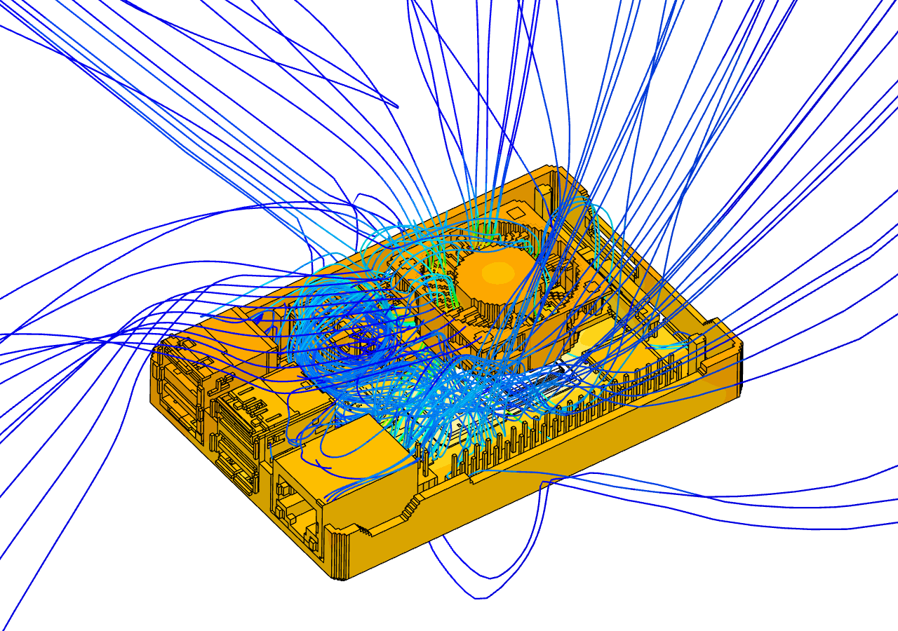
A section view of the domain provides additional insights into flow fields.

1. Toggle off Parts color and toggle on ‘Cutting Plane’.
2. Choose the ‘Z’ axis for orientation. Verify the position to ensure the plane is correctly located.
3. Set Coloring to ‘Velocity Magnitude’.
4. Toggle on ‘Vectors’.
5. Set Scaling factor to ‘0.04’ and Grid Spacing to ‘0.005’.
6. Enable ‘Project vectors onto plane’.

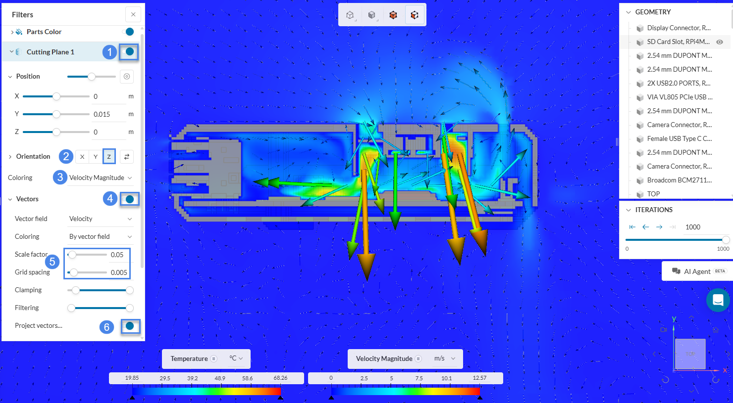
This visualization reveals the impact of the momentum source, showing how the fan actively draws air into the enclosure to drive the cooling cycle.

5.4 Streamlines

Add a ‘Particle Trace’ filter to view streamlines. This tutorial uses the cutting plane as the seed face to focus on internal airflow. Hide the flow region, activate the cutting plane, and select a region within the equipment as the seed face.

1. Select the ‘Particle trace’ icon from the filter section.
2. Select the center of the cutting plane as the seed region.
3. Adjust horizontal and vertical seeds to cover the inlet areas.
4. Set Spacing to ‘0.003’.
5. Set size to ‘0.00015’.

After hiding the flow region, cutting plane, and enclosure top, the result should resemble Figure 36.

For an overview of post-processing capabilities, consult this documentation.

Congratulations! The tutorial is complete!

Last updated: February 12th, 2026