How to Set Orthotropic Thermal Parameters?

This knowledge base article explains how to set orthotropic thermal conductivity in a Conjugate Heat Transfer v2.0 analysis and the configuration of the unit vectors.

Printed Circuit Board (PCB) Background

Assigning realistic material properties is important to achieve accurate simulation results. Isotropic material properties mean that the properties are independent of the direction, whereas anisotropic materials have direction-dependent properties.

A typical Printed Circuit Board (PCB) is made up of layers of plastic (usually FR4), with copper layers in between. This component is unique as it is not a single type of material, but for simulation purposes, it is treated as such.

PCBs are characterized by an anisotropic thermal conductivity, so it is important to take this into account for calculations. The in-plane thermal conductivity is usually very high (around 20 \(W/(m.K)\)), whereas the cross-plane conductivity is often below 1 \(W/(m.K)\). If you are interested in learning how to calculate the anisotropic thermal conductivity values in PCBs, check this article.

Solution

In SimScale, the Conductivity type settings are found within the solid Materials tab in the Simulation Tree. A total of three options are available:

• Isotropic
• Orthotropic
• Cross-plane orthotropic

Find below how to configure the Orthotropic and Cross-plane orthotropic settings.

Orthotropic

With Orthotropic settings, the user can define a different Thermal conductivity for each direction.

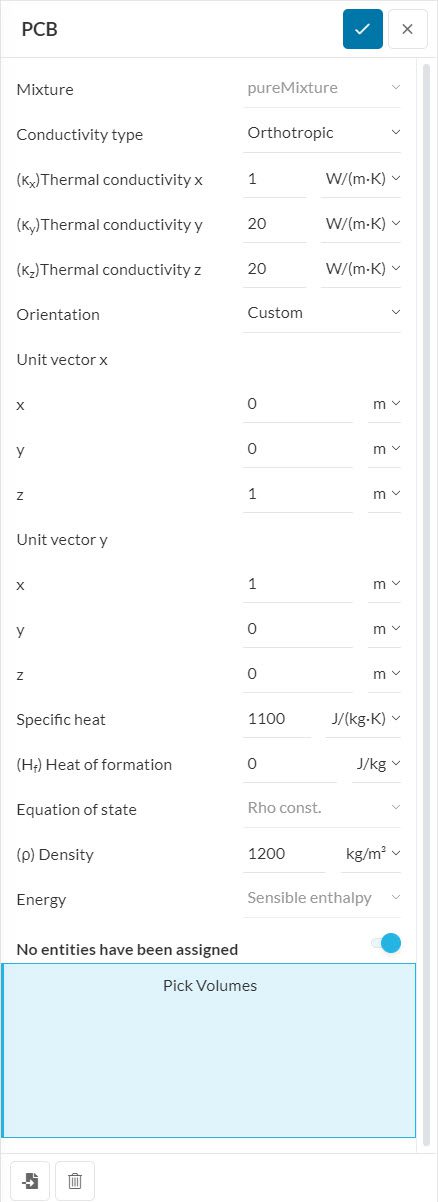
Furthermore, the Orientation can be Cartesian or Custom. With Cartesian, the global coordinate system is used to determine the x, y, and z-directions.

In the case of a Custom orientation, the user sets a local coordinate system by defining the local Unit vector x and Unit vector y, which must be orthogonal to each other. Please note that the definition of the local unit vectors is done with respect to the global coordinate system.

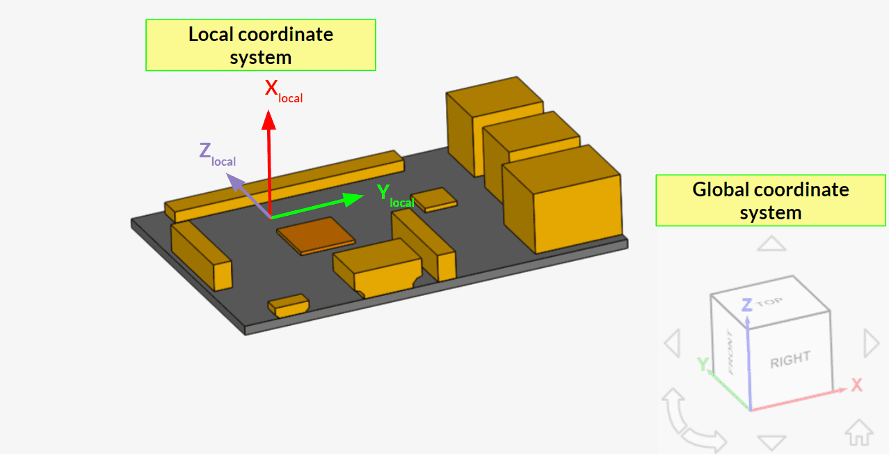
For example, Figure 2 below shows the local coordinate system based on the following input:

• Unit vector x: (0, 0, 1)
• Unit vector y: (1, 0, 0)
• The Unit vector z is automatically set by the algorithm, being perpendicular to the first 2 vectors

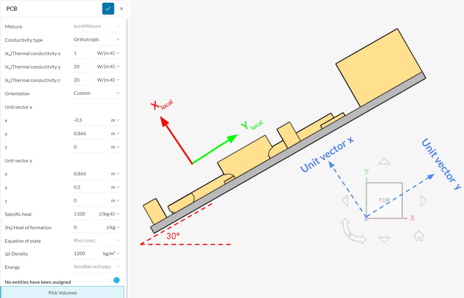
This formulation gives the user flexibility in setting their local coordinate system. For example, it is possible to define angled relative coordinate systems, as in Figure 3:

Cross-Plane Orthotropic

For a Cross-plane orthotropic configuration, the user needs to define the in-plane and cross-plane thermal conductivities. Similarly to the orthotropic approach, it is possible to choose between Cartesian and Custom Orientation.

When using Cartesian, the cross-plane direction is always taken as the global z-direction, whereas the in-plane conductivity acts in the global x and y-directions.

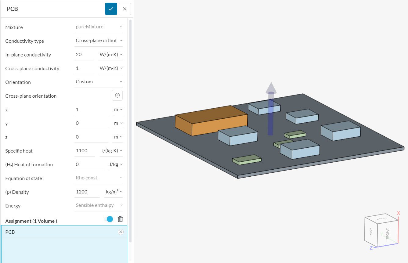
For a Custom orientation, the user needs to define the direction where the cross-plane thermal conductivity acts. Finally, the in-plane conductivity acts in a plane that is orthogonal to the cross-plane direction.

Figure 4 shows an example of a cross-plane orthotropic configuration. In the viewer, an arrow will indicate the cross-plane direction based on the input.

With the orthotropic models for the thermal conductivity, users can simulate their PCB materials much more accurately.

Expected Outcome

To show how different the results can be, the simple electronic device model is tested with isotropic and orthotropic PCB materials. For the isotropic simulation, a Thermal conductivity of 20 \(W/(m.K)\) is defined.

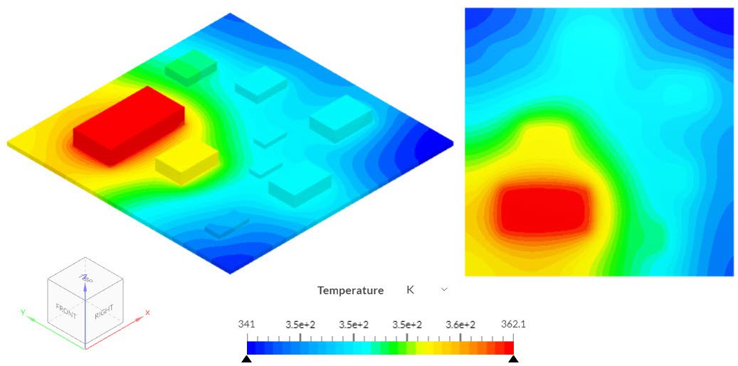
Since the isotropic PCB has a high thermal conductivity in the cross-plane direction, the bottom of the PCB is also under a high temperature. When solving the same simulation, but defining an In-plane conductivity of 20 \(W/(m.K)\) and a Cross-plane conductivity of 0.5 \(W/(m.K)\) in the z-direction, the following results are obtained:

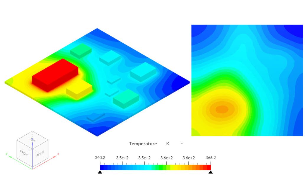
Due to the lower thermal conductivity in the cross-plane direction, a larger temperature gradient develops across the PCB. As a result, the processors reach slightly higher temperatures, since the conductivity in the cross-plane direction is compromised.