Advanced Tutorial: Fluid Flow Simulation Through a Water Turbine
This tutorial showcases how to use SimScale to run an incompressible fluid simulation on a water turbine using rotating zones. The complexity of this use case results from the requirement of modeling a rotating region.
Simulations involving rotating regions require a few additional steps during CAD preparation and simulation setup. We will cover the entire workflow in this tutorial.
This tutorial teaches how to:
- Set up and run an incompressible water turbine simulation, making use of a rotating zone;
- Assign boundary conditions, material, and other properties to the simulation;
- Mesh with SimScale’s standard meshing algorithm.
We are following the typical SimScale workflow:
- Prepare the CAD model for the simulation;
- Set up the simulation;
- Create the mesh;
- Run the simulation and analyze the results.
1. Prepare the CAD Model and Select the Analysis Type
To begin, click on the button below. It will copy the tutorial project containing the geometry into your Workbench.
The following picture demonstrates what is visible after importing the tutorial project.
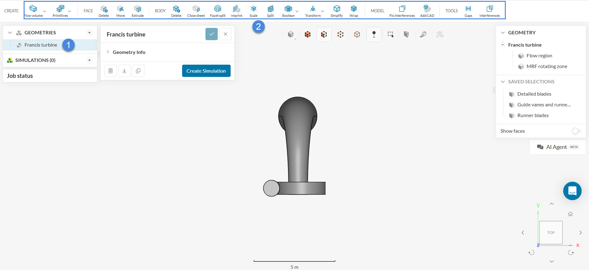
The Simulation contains one geometry that consists of the Flow region of a Francis turbine and the MRF rotating zone.
Did you know?
Water turbines operate by removing kinetic and potential energy from the flow and converting it into mechanical torque on a shaft.
Water pumps work in the exact opposite way. By inputting mechanical energy, in the form of torque on a shaft, pumps can pressurize the water flow.
1.1 Geometry Preparation
The imported geometry for this tutorial is ready for CFD simulations. Please note that it doesn’t contain any of the solid walls of the turbine. For this kind of analysis, only the flow region and rotating zone are necessary. If we needed to prepare the flow region ourselves, and to create the flow region as well, we would use the CAD environment. To modify a CAD model, simply select the geometry from the list—the available CAD operations will then appear in the top toolbar. You can either work directly on the original model or create a duplicate and apply your changes to the copy.
In case you are interested in the workflow to prepare your turbine design for a simulation with rotating zones, consider checking the following articles:
Creating a Cylinder in the Edit in CAD Mode
Did you know? Rotating zones can also be created on the SimScale platform using the CAD mode. Check out this acticle in order to learn how to create a cylinder in the Edit in CAD mode.
1.2 Create the Simulation
To start the simulation setup process select the Francis turbine geometry to access further options.
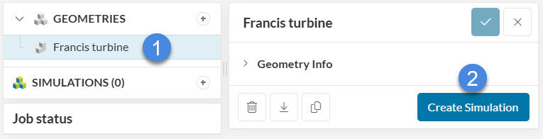
Hitting the ‘Create Simulation’ button leads to the simulation type selection widget:
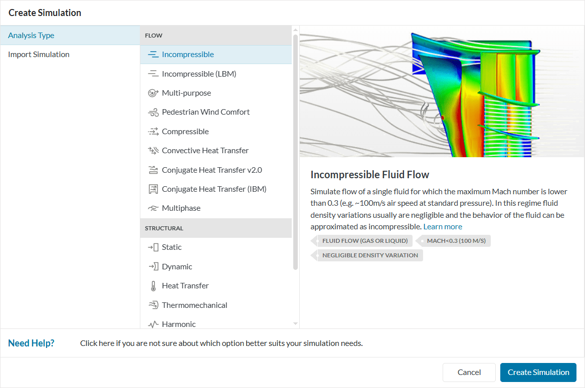
Choose ‘Incompressible’ as the analysis type and confirm the selection by clicking on ‘Create Simulation‘.
2. Assigning the Material and Boundary Conditions
The following picture shows an overview of the boundary conditions.
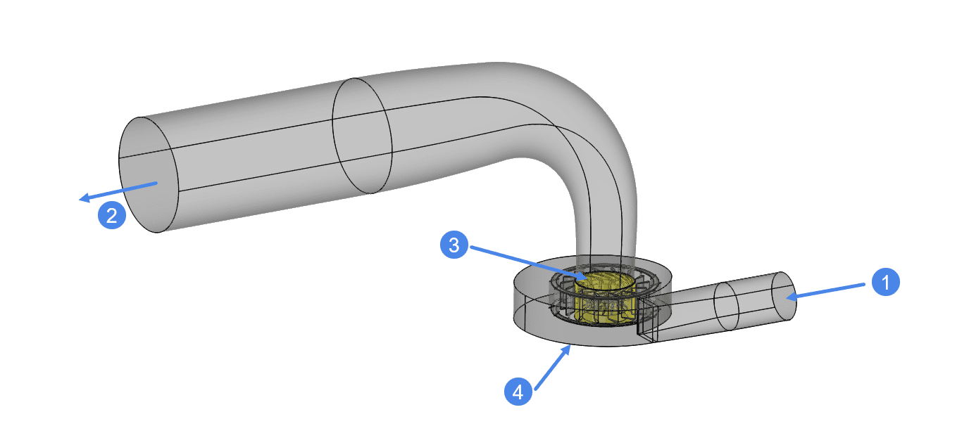
- Volumetric Flowrate Inlet \( \dot U= 16 \frac{m^3}{s} \)
- Gauge Pressure Outlet \(0 Pa\)
- MRF rotating zone \(36.61 \frac{rad}{s}\)
- Rotating Wall \( 0 \frac{rad}{s} \)
Did you know?
The entire volume inside the MRF rotating zone is spinning at a specified rotational velocity.
In case the rotating zone intersects a surface that shouldn’t be spinning, you can create a rotating wall boundary condition for this face, specifying a rotational velocity of 0. This will prevent the intersected parts from spinning.
For example, in our geometry, one face that shouldn’t spin is intersected by the rotating zone:
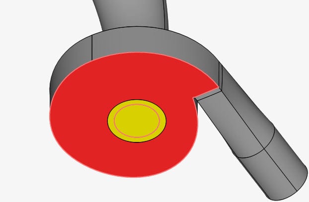
Figure 6: MRF rotating zone (in yellow) partially intersecting a surface (in red).
Later on, in this tutorial, the face highlighted in red will receive a rotating wall boundary condition, with a 0 \(rad/s\) rotational velocity.
2.1 Define a Material
This simulation will use water as fluid. Therefore click on the ‘+ button ‘ next to materials. In doing so, the SimScale fluid material library opens, as shown in the figure below:
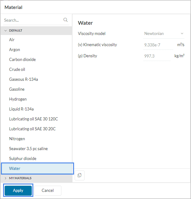
Select ‘Water’ and click ‘Apply’. Keep the default values, and assign the entire Flow region to it.
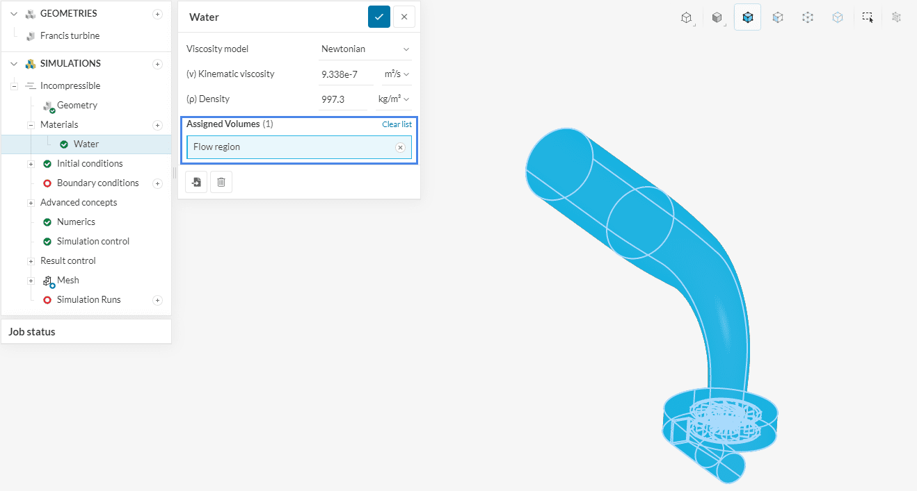
The MRF rotating zone volume is not assigned to any material.
2.2 Assign the Boundary Conditions
In the next step, boundary conditions need to be assigned as shown in Figure 5. We need to set up and assign a velocity inlet, a pressure outlet, a rotating wall, and a rotating zone.
2.2.1 Velocity Inlet
Click on the ‘+ button ‘ next to boundary conditions. A drop-down menu will appear, where one can choose between different boundary conditions.
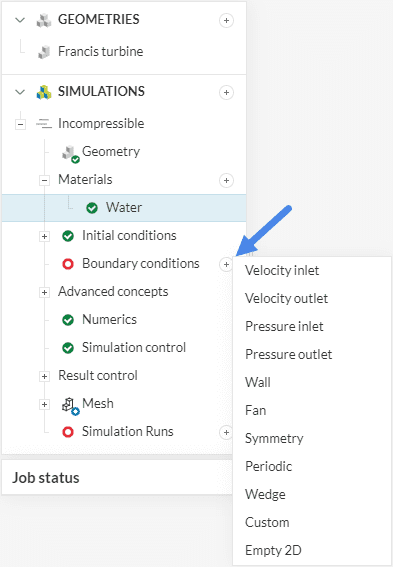
After selecting ‘Velocity inlet’, we have to specify some parameters and assign faces. Please proceed as below:
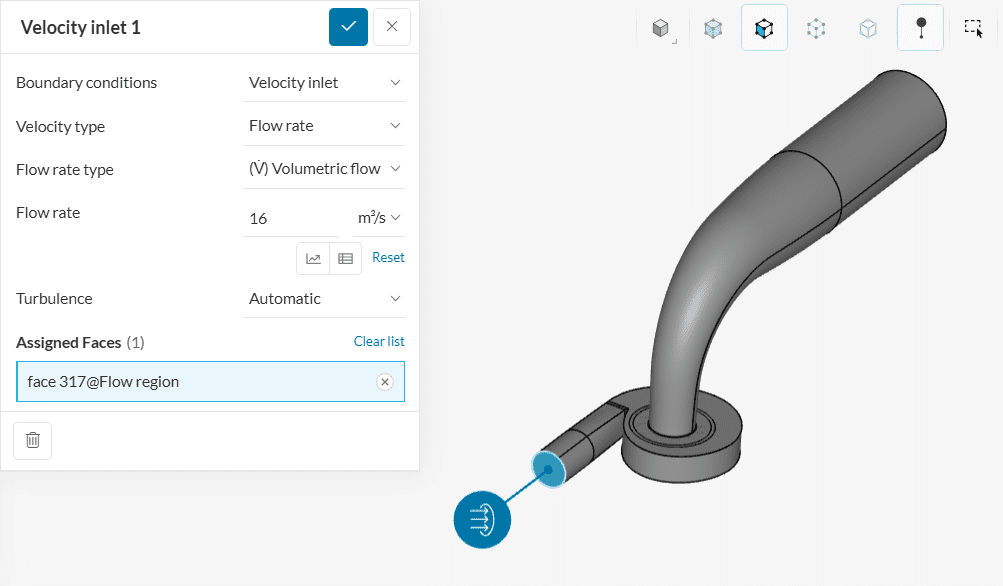
A volumetric flow rate of ’16’ \( \frac{m^3}{s}\) of water will enter the domain through the inlet face.
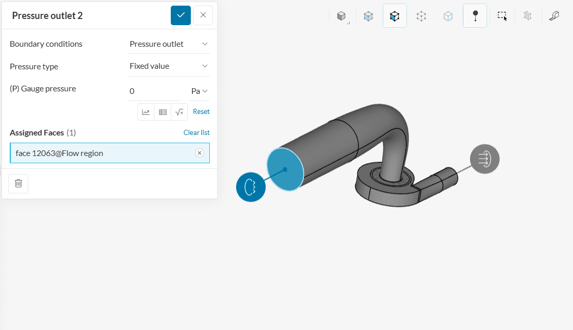
2.2.2 Pressure Outlet
The next one will be a pressure outlet at the outlet face. Make sure (P) Gauge pressure is set to a Fixed value of ‘0’ \(Pa\).
Did you know?
After going through the turbine runner, water exits through a section named draft tube. The purpose of this tube is to slow down the flux, converting kinetic energy into potential energy.
The draft tube should be carefully designed, as it is directly related to kinetic energy loss at the outlet.
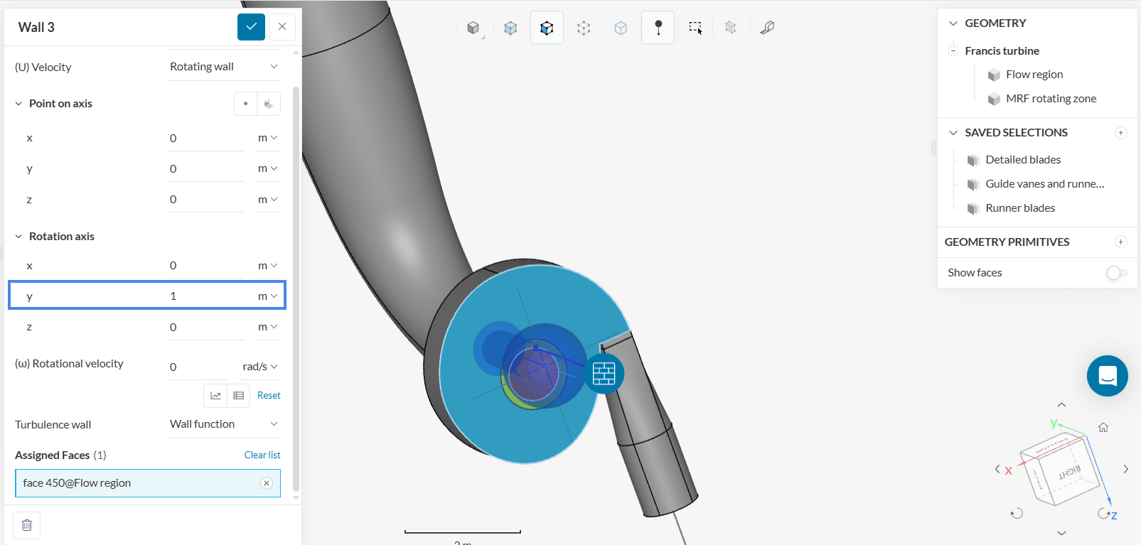
2.2.3 Rotating Wall
As previously described, one of the faces receives a rotating wall boundary condition using Figure 9. To achieve this, create a new boundary condition and choose ‘Wall’. Set it up as shown below:
Remaining Walls / Surfaces
For the remaining surface / walls no boundary conditions have to be created, as SimScale will automaticly assign a no slip boundary condition to all surfaces without a user defined boundary condition.
2.3 Advanced Concepts: Creating a Rotating Zone
In the left-hand side panel, navigate to Advanced concepts. Click on the ‘+’ button next to Rotating zones and select ‘MRF rotating zone’. Define the MRF zone as shown:
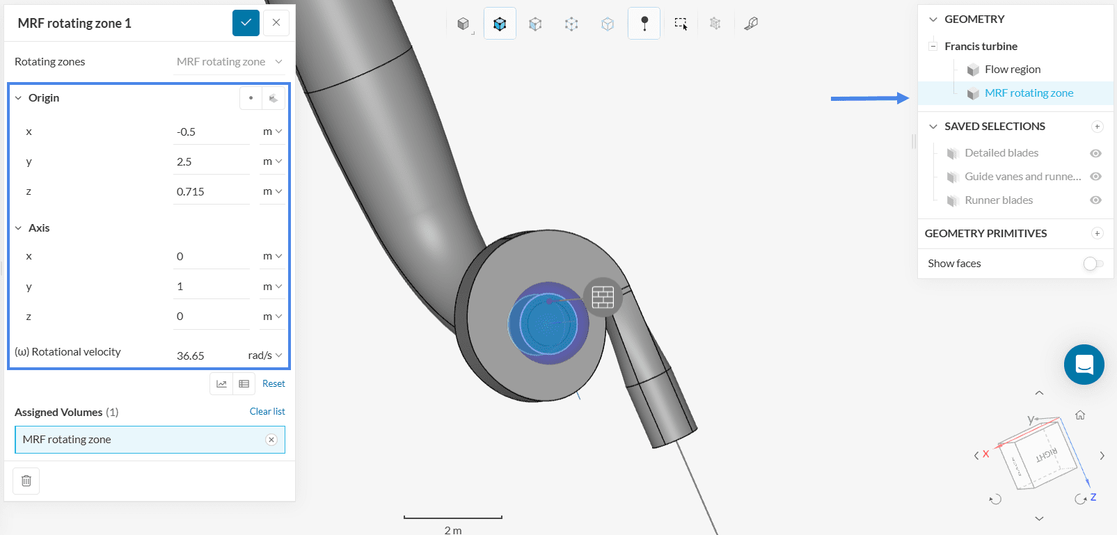
Did you know?
MRF Rotating zones are chosen in this project, as we are running a steady-state simulation.
If we were calculating a transient problem, we would need to choose AMI Rotating Zone.
This article provides more information about the difference between MRF and AMI Rotating Zones.
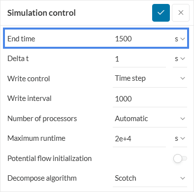
2.4 Numerics & Simulation Control
The default settings for the Numerics are enough for this turbine simulation. In fact, it is recommended that the user doesn’t alter the numerical settings unless they are well understood and need to be adjusted.
We will, however, increase the End time to ‘1500’ seconds.
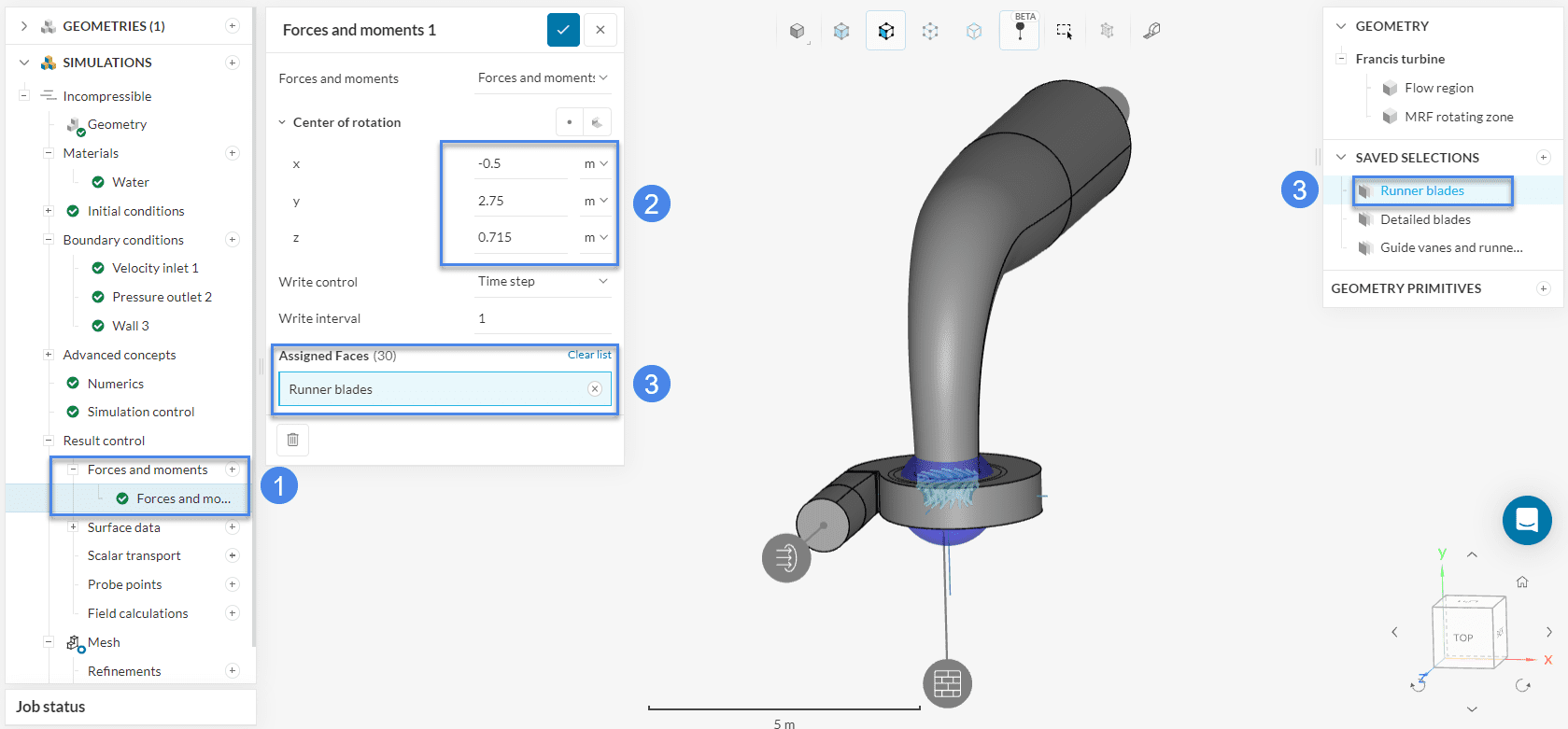
2.4 Result Control
Under result control, users can specify a variety of monitors, such as area averages and probe points. These are particularly useful to assess convergence and the reliability of the results. For now, let’s set up 2 result controls – we will take a look at the results later on during the tutorial.
To assess the force and torque applied on the turbine runner blades please set a ‘Forces and moments’ control item. Assign it to a pre-defined saved selection named ‘Runner blades’:
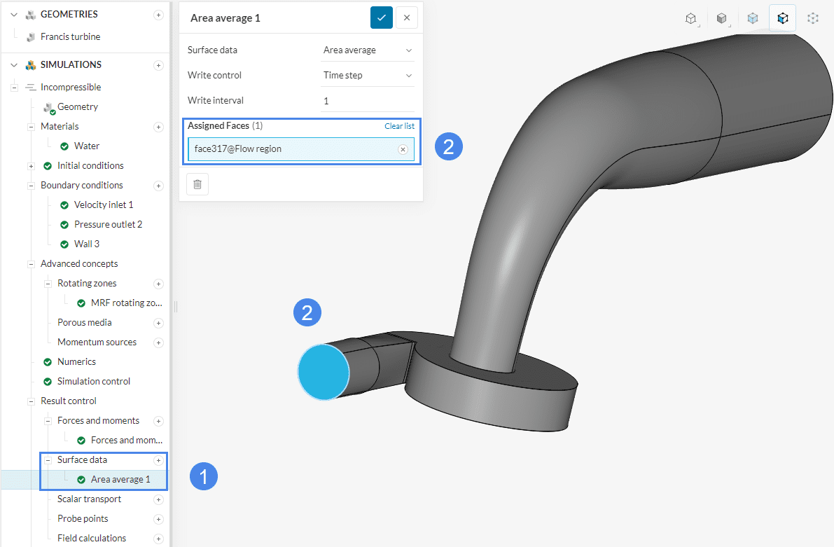
Another important characteristic of a pump is the pressure drop. Since the outlet is set to 0 \(Pa\) the pressure at the inlet directly displays the pressure drop of the pump. Therefore create a second control item. Click on the ‘+ button’ next to Surface data. Create an ‘Area average’ control for the inlet, as shown in the picture below.
3. Mesh
To create the mesh, the Standard algorithm will be used with the standard settings. In addition to the standard settings, a few mesh refinements will be created to ensure that the features of the blade and fins will be accurately captured.
Did you know?
It’s necessary to define cell zones whenever we want to apply a specific property, such as a rotating motion, to a subset of cells.
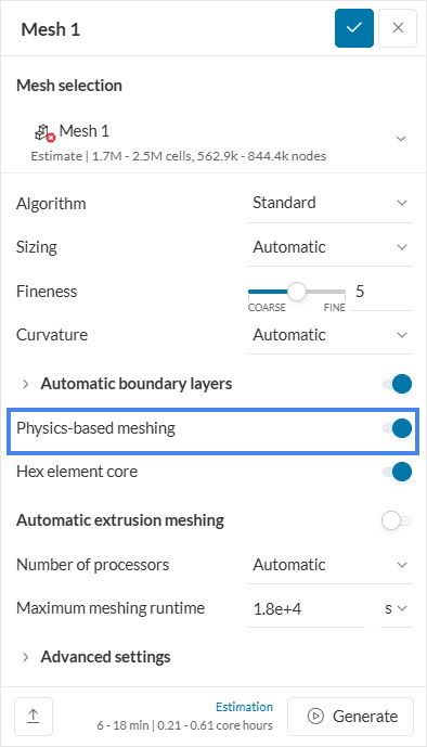
Whenever Physics-based meshing is enabled for the standard mesher, the algorithm automatically creates the necessary cell zones. Since physics-based meshing is enabled in this tutorial (see Figure 17), we don’t have to worry about the cell zone definition.
In case you are using a different mesher, the rotating zones documentation page provides alternative workflows for the cell zone definition.
3.1 Mesh Refinements
a. Surface custom sizing 1
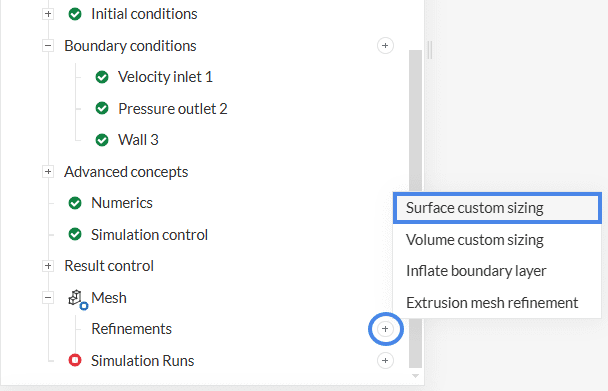
To create a mesh refinement, click on the ‘+’ next to Refinements. Choose the ‘Surface custom sizing’ from the drop-down window.
With a surface refinement, it’s possible to prescribe a fineness level under automatic sizing method for selected entities. Proceed as below to set up the first refinement:
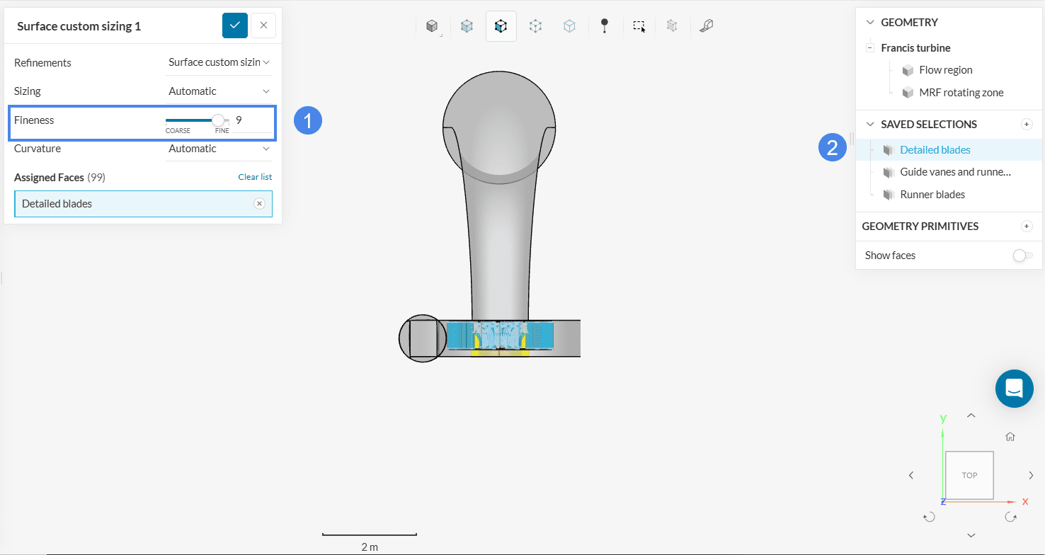
Set fineness to ‘9’. To save time, you can assign this first surface refinement to the saved selection named ‘Detailed blades’.
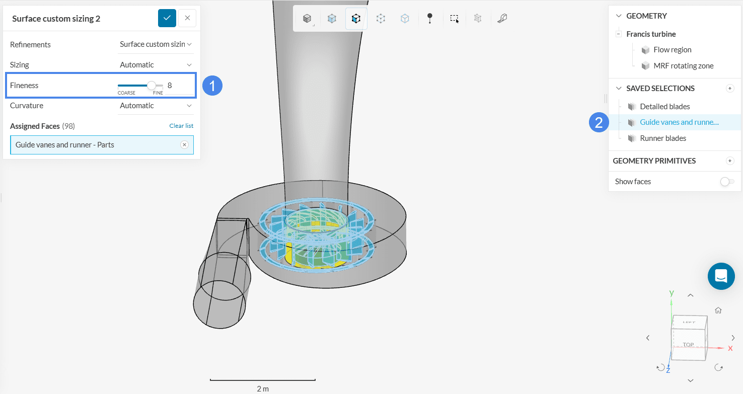
b. Surface custom sizing 2
Create yet another ‘Surface custom sizing’ refinement. This time we will select geometry parts that don’t require as much refinement. Adjust fineness to ‘8’ and assign it to ‘Guide vanes and runner-Parts’ saved selection:
4. Start the Simulation
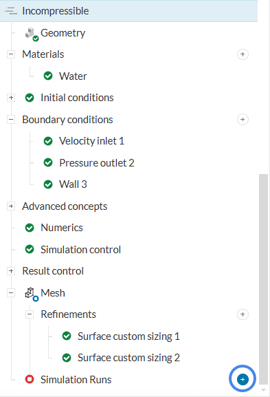
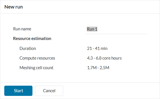
Click on the ‘+ button ‘ next to Simulation Runs.
Now you can hit the ‘Start’ button to begin the simulation.
4.1 Observing the Mesh
Mesh is generated as a part of the simulation run and need not be generated separately. The generated mesh can be observed under Mesh while the details can be seen under Event log.
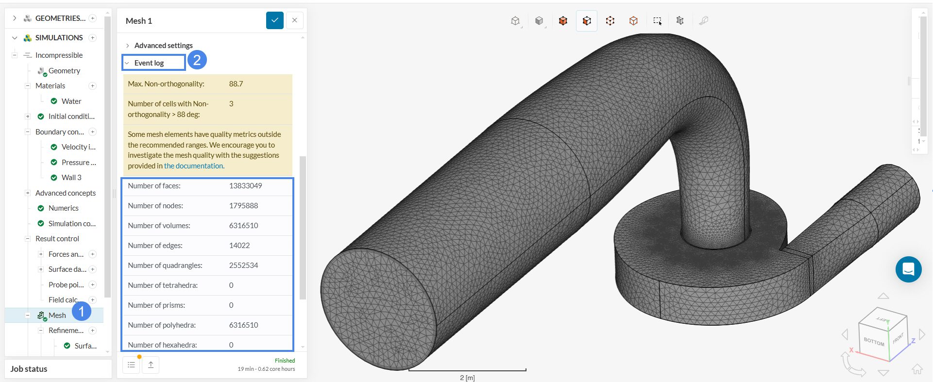
For more insights on mesh quality assessment, please check this page.
Did you know?
You can also select single faces of the geometry and hide them. This way, you can inspect inner surfaces.
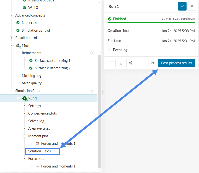
4.2 Accessing the Results
While the results are being calculated you can already have a look at the intermediate results in the post-processor by clicking on Solution Fields. They are being updated in real time!
After about an hour, the turbine simulation finishes running.
5. Post-Processing of a Turbine Simulation
5.1 Pressure Drop
One of the most important parameters to observe when evaluating the performance of a water turbine is how much the pressure drops after the water has flown through the turbine. You can calculate the pressure drop by subtracting the inlet pressure from the outlet pressure.
Because you have added an Area average output for the inlet and defined a pressure outlet with 0 \(Pa\), only the pressure at the inlet is required to calculate the pressure drop.
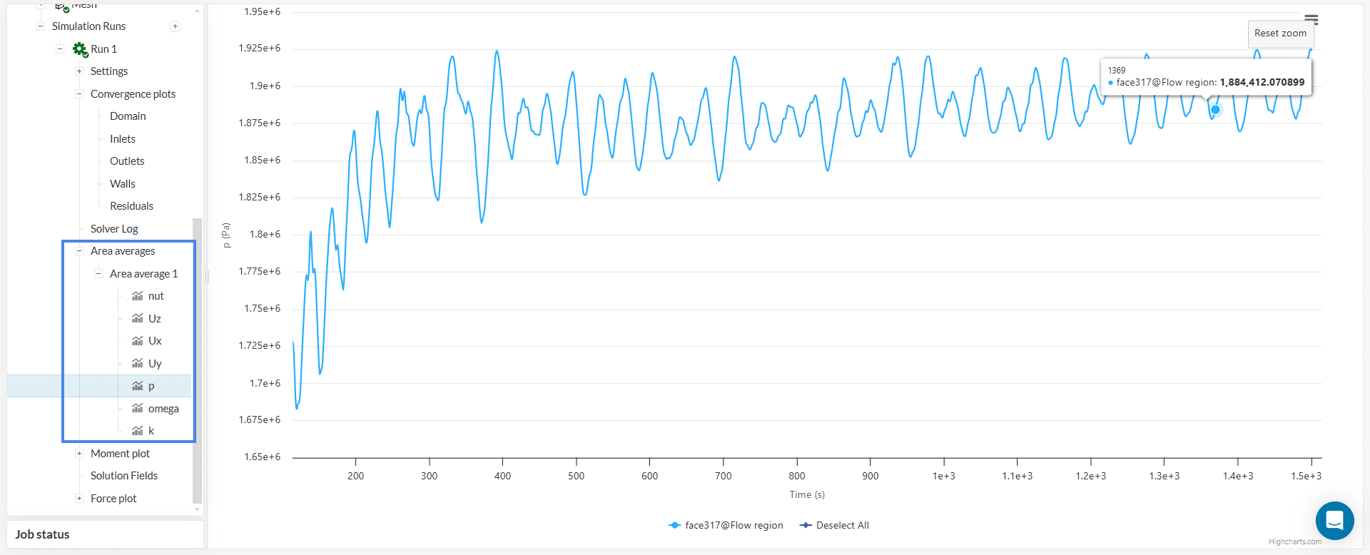
As you can see from the figure above, the pressure still has some fluctuations therefore the average of the last values should be calculated. For example, calculate the average from time step 1000 to 1500 which is approximately 1.894 \(MPa\). So, the pressure drop due to the turbine is approximately 1.894 \(MPa\).
Find more ways to calculate the pressure drop here.
Zooming into Plots
To observe the plots from one iteration to other, for example, iteration 100 to 1500, see Figure 25, double tap on an iteration and drag it up to the intended iteration. Click on ‘Reset zoom’ to zoom out to the original layout.
Fluctuation of a result control Item
Even though the simulation was run in steady-state, transient effects can still occur. Have a look at this article on how to detect transient effects in a steady state simulation.
5.2 Forces and Moments on the Turbine Blades
The Forces and moments results are of particular interest in a simulation with a turbine. The runner of our turbine was rotating around the y-axis. Hence, let’s inspect the resulting pressure forces and the torque generated around said axis:
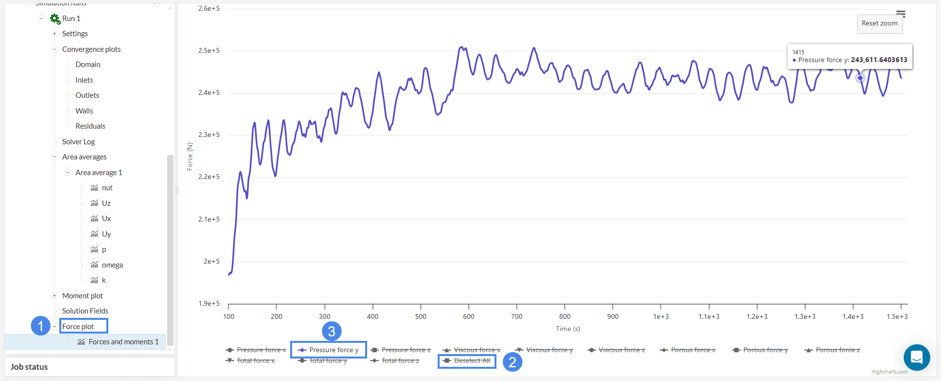
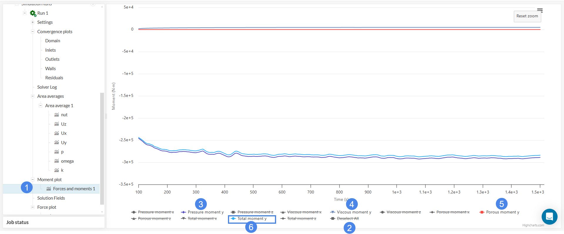
Did you know?
The resulting torque on the blades is given by a sum of pressure, viscous and porous moments around the rotation axis or the total moment about y axis
In this simulation, close to 284000 \(N.m\) of torque is generated about the y-axis of the turbine.
5.3 Particle Traces
Streamlines can be a great tool to visualize flow patterns, especially in rotating machinery applications. Follow the steps below to show the flow streamlines inside the turbine:
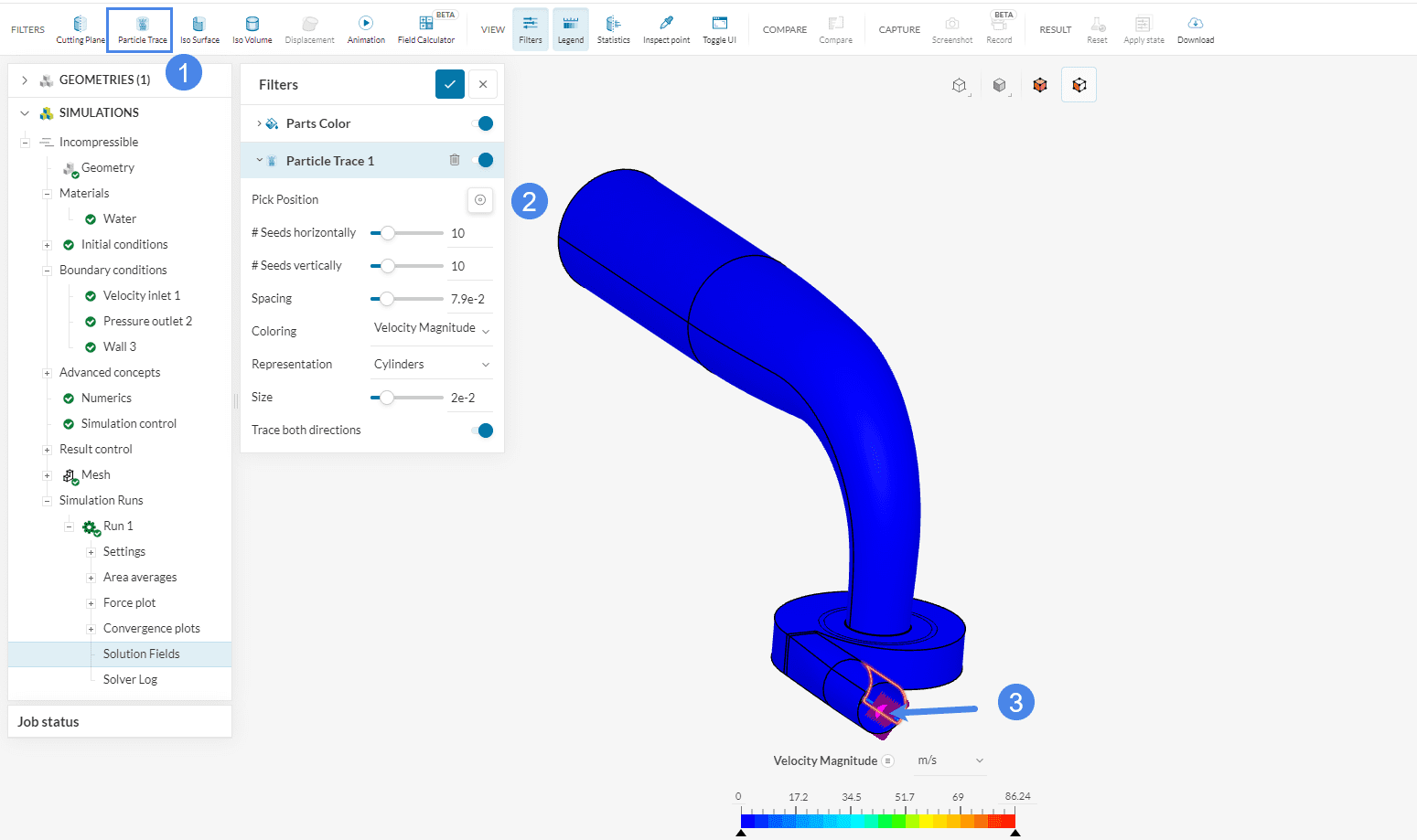
- Remove any predefined filters and click on the ‘Particle Trace’ on the top filters ribbon.
- Choose the inlet as a seed for the traces.
Now repeat the process, but this time select the outlet as a seed face.
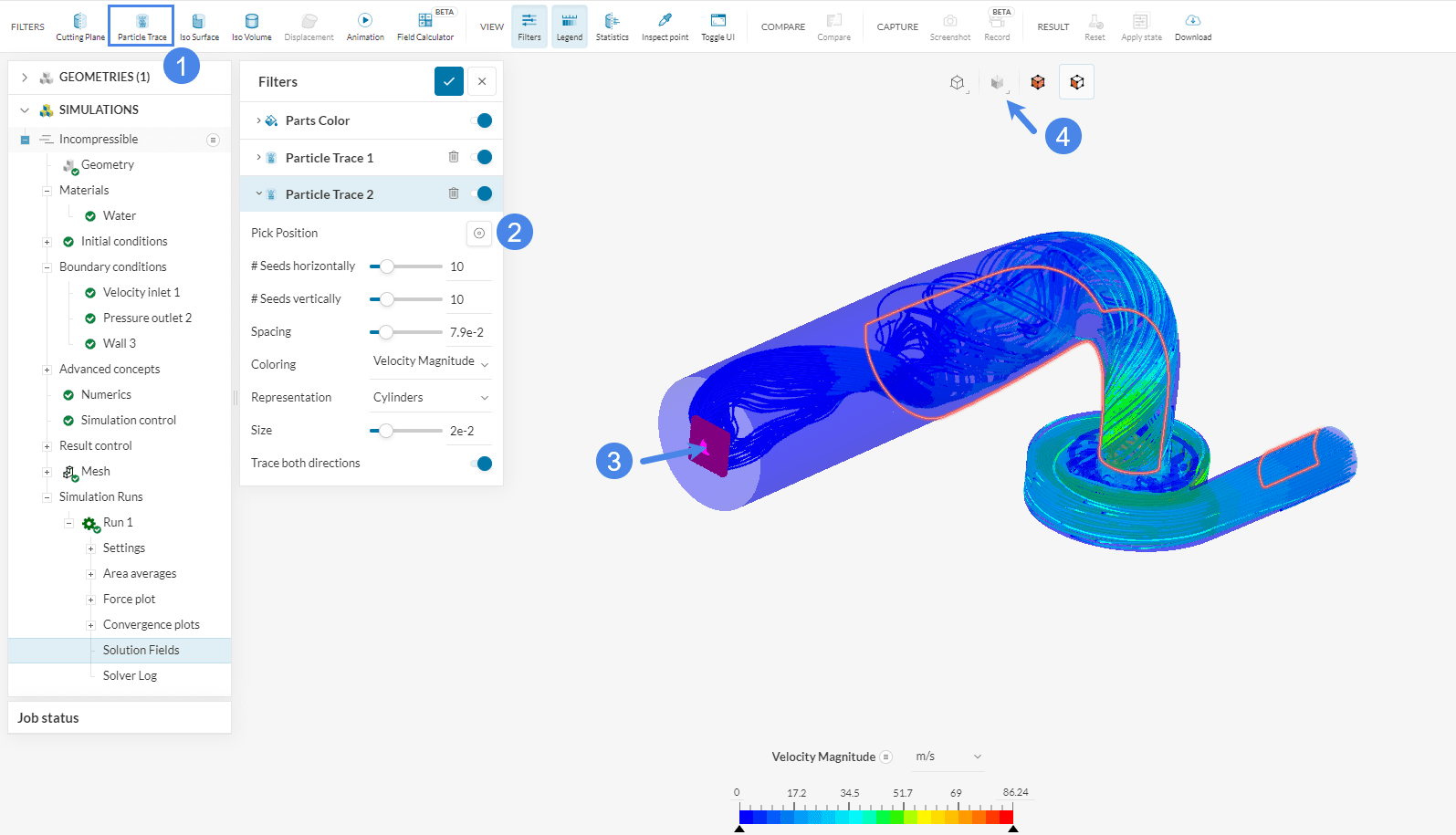
After the traces are created, you can adjust the render mode to ‘Translucent surfaces’ to give a better view of the flow. We can see that the flow follows a circular motion in the outlet region due to the rotatory motion of the turbine.
5.4 Cutting Planes
To get more details on the flow behavior inside the turbine, hide the Parts Color and create a Cutting Plane filter.
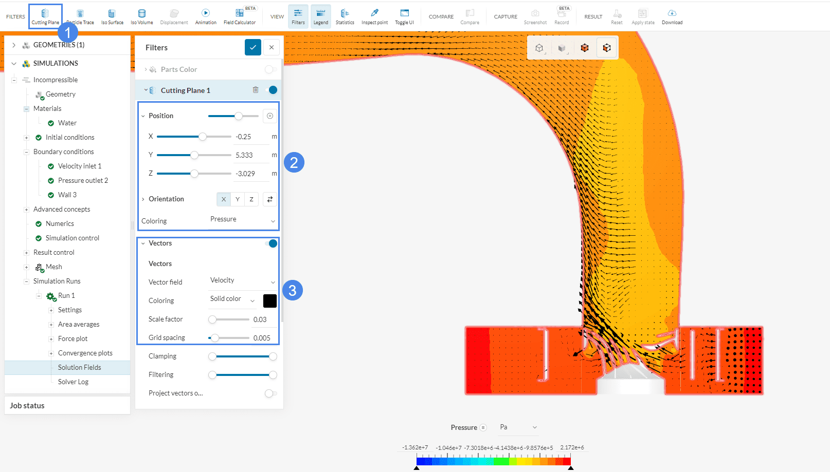
- Create a ‘Cutting plane’ filter using the top ribbon.
- In the configuration window, change the Position of the cutting plane to ‘-0.25, 5.333, -3.029’. Furthermore, adjust the Orientation of the cutting plane to the ‘X’ direction. The Coloring of the plane is ‘Pressure’.
- Turn on the Vectors toggle and change the Coloring to a solid color and choose the color black. Finally, reduce the Scale factor of the vectors to ‘0.03’ and the Grid spacing to ‘0.005’.
From the figure above, you can see how the water pressure drops when flowing inside the turbine and decreases even more after flowing to the outlet. You can also see how the blades are affecting the flow by adjusting the position and orientation accordingly. Please follow the instructions below:
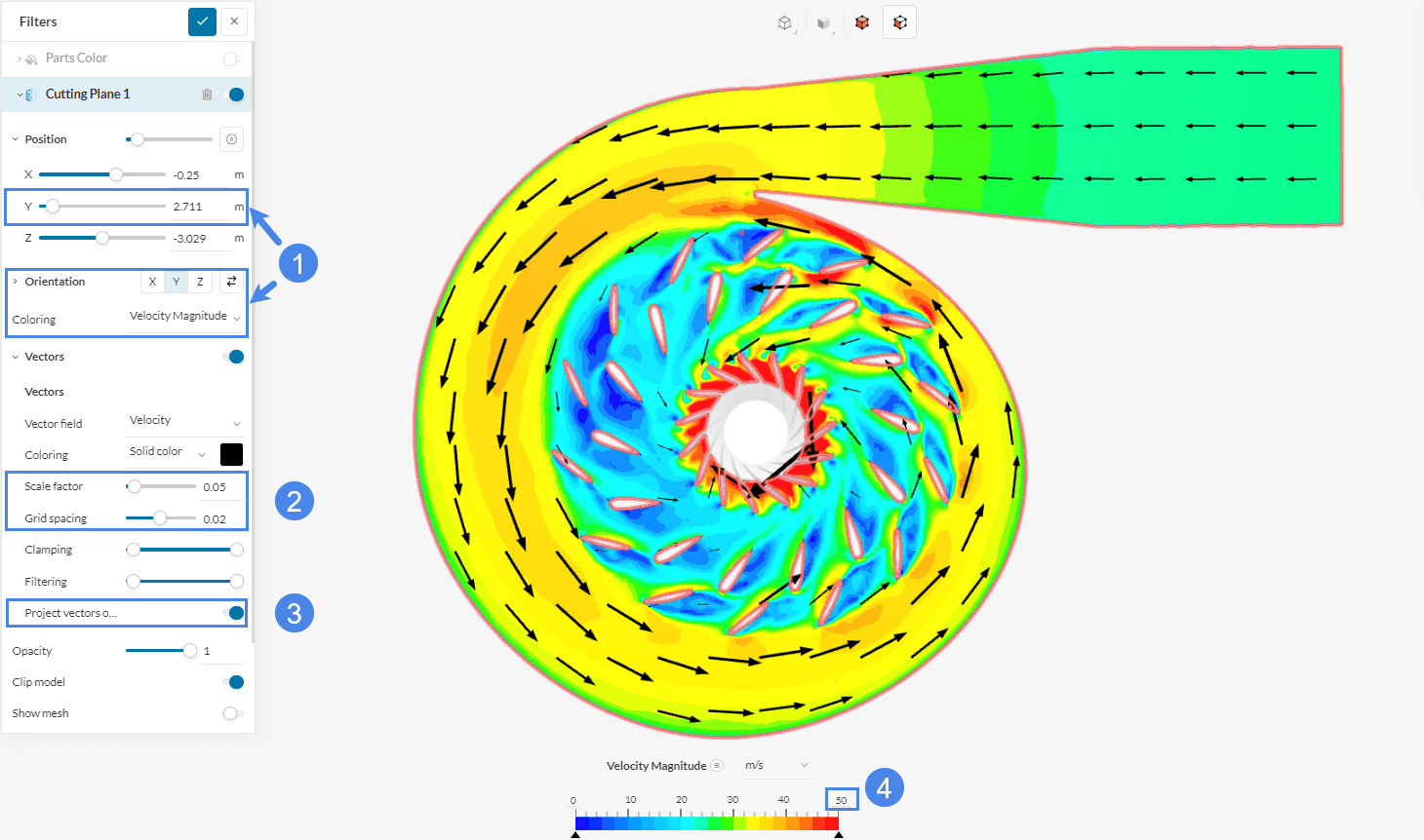
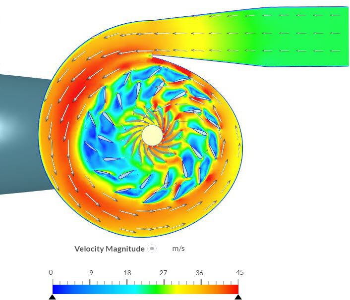
- Change the Position of the cutting plane to ‘-0.25, 2.771, -3.029’. Furthermore, adjust the Orientation of the cutting plane to the ‘Y’ direction. The Coloring of the plane is ‘Velocity Magnitude’.
- Adjust the Scale factor of the vectors to ‘0.05’ and the Grid spacing to ‘0.02’.
- Enable the Project vectors onto plane option.
- Double-click on the higher-end value of the velocity magnitude and reduce it to ’50’. The value of 50 is chosen since the majority of the flow lies within this value and as a result the contours are more defined.
In this view, you can get insights into how the blades and guide vanes are affecting the flow, allowing for optimizations in the design.
Analyze your results with the SimScale post-processor. Have a look at our post-processing guide to learn how to use the post-processor.
Note
If you have questions or suggestions, please reach out either via the forum or contact us directly.
Last updated: April 6th, 2026
Did this article solve your issue?
How can we do better?
We appreciate and value your feedback.


