How to Detect Transient Behavior in Steady-State Simulations?

This article aims to explain and show how to detect transient flow characteristics in a steady-state simulation.

What Are Steady-State Simulations?

In a CFD simulation, a steady-state is considered when all flow characteristics such as velocity, pressure, or temperature are constant. Constant means that the flow characteristics of the current time step do not differ from the flow characteristics of the previous time step and will not change for any further time steps. A steady-state solution can therefore be expressed with the following formula:

$$ \lim \limits_{n \to \infty} p_{n} \ – \ p_{n-1} = 0 \tag{1} $$

In a steady-state, with constant flow characteristics, the simulation is being considered as converged. The following article shows how to decide if your simulation converges or not.

How to Check Convergence of a CFD Simulation?

Transient Behaviour in Steady-State Simulation

For some geometry or flow conditions, the flow characteristics result in a transient solution, therefore a steady-state condition cannot be achieved. An example of this can be seen in Animation 1 where the front face of the building is at 45° angle of attack. The flow around this building detaches, which creates a turbulent wake area for which there is no steady-state solution.

Another example of a case where only a transient solution exists is the flow over a cylinder for certain Reynolds numbers. For the right flow conditions, a Kármán vortex street can occur and therefore a steady-state solution for the cylinder can not be achieved. Such Kármán vortex street can be seen in Animation 2.

Check Result Control Items and Residuals

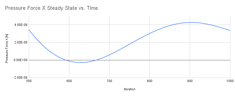
One way to detect transient effects in a steady-state analysis is to check for either transient residuals or transient results of a result control item. In Figure 1 the surface pressure force on a cylinder is displayed for each iteration of a steady-state analysis. We can see that the surface pressure force is not converging to one solution, but rather is oscillating. This tells us that transient behavior is occurring and therefore the simulation should be checked for a transient solution.

To check for a transient solution, the same case has been simulated, changing the time dependency from steady-state to transient. You can change the time dependency of a simulation in the global settings item of the simulation tree. In Figure 2 below we can have a look at the pressure force for the same cylinder, but now for a transient simulation.

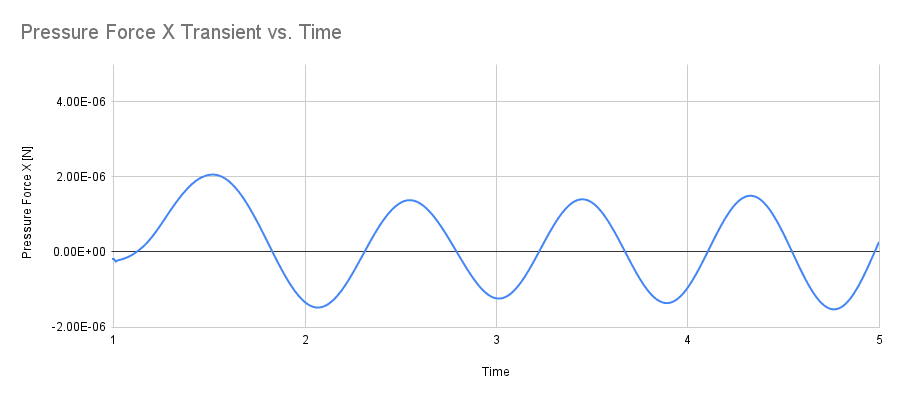
The result of the pressure force of the transient solution oscillates with a frequency of 0.88 \(Hz\). Compared to the stationary result, we can observe that the pressure force can also occur in the negative x-direction. The result shows us how important it can be to correctly detect transient effects in steady-state simulations. Below are more examples of residual and result control plots to show how to detect transient behavior in steady-state simulations.

Further Examples

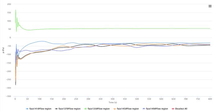
1. Figure 3 shows the pressure for the different surfaces of a building at an angle of attack of 45°. Although the pressure for some surfaces converges to a steady-state, the pressure for other surfaces does not, indicating that a transient solution might exist for this case.

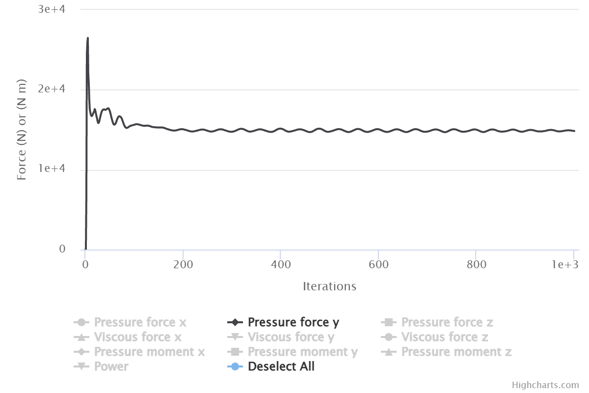
2. Figure 4 shows the pressure force in the flow direction on a butterfly valve. Here it can be seen that the result does not converge to a single value, but oscillates at a constant rate. This shows that there is no steady-state solution in this case and a transient simulation should be performed.