With the convective heat flux boundary condition, a linear heat transfer model is applied between the boundary entities and the external environment. This is useful to model general heat losses or gains such as those due to natural/forced convection or conduction with adjacent bodies of relatively constant temperature.
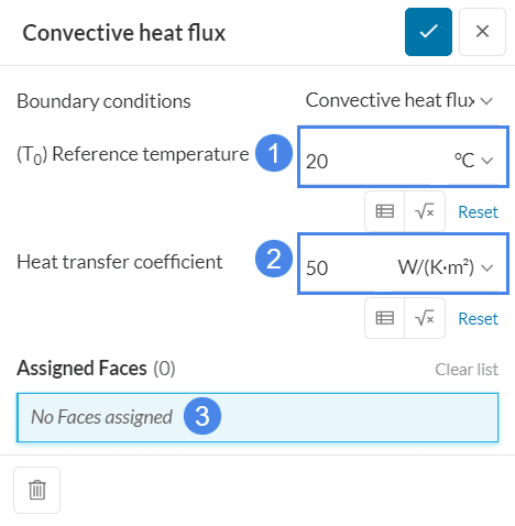
Figure 1: Convective heat flux boundary condition panel. Enter the desired reference temperature and heat transfer coefficient, or select the variable button to input a function or table.
The parameters of the boundary condition are:
Reference temperature: Temperature of the environment, used to compute the boundary heat transfer.
Heat transfer coefficient: Proportionality value used to compute the boundary heat transfer, with units of power \((W, Btu/h)\) divided by units of temperature \((K, °C, °F)\) and area \((m^2, in^2)\)
Assignment: Set of faces where the convective heat flux value will be applied.
Function or Table input
The values for the reference temperature and heat transfer coefficient in the settings panel for the convective heat flux boundary condition can also be input using the function or table capability.
Supported Analysis Types
The following analysis types support the usage of this boundary condition:
\( \kappa \) is the thermal conductivity of the material,
\( \nabla T \) is the local temperature gradient,
\( \vec{n} \) is the area normal vector of the element boundary surface,
\( h \) is the convection heat transfer coefficient,
\( T \) is the local temperature.
\( T_{ref} \) is the external reference temperature, and
Variable Convective Heat Flux
Variable heat flux values can be specified with the use of the formula or table inputs for the reference temperature and/or the heat transfer coefficient. The allowed functions are:
Time-dependent: The parameters vary with respect to time (variable t) in a transient heat transfer, nonlinear static or dynamic thermomechanical simulation. This is useful, for instance, to ramp up the load from zero in nonlinear simulations, where a sudden application of load leads to numerical divergence, or to define heat transfer curves. This option is available for both formula and table inputs.
Coordinate-dependent: The parameters vary with respect to the position in space (variables X, Y, Z). This is useful for applying known heat transfer gradients on the boundary faces. If the heat flux only depends on 1 variable, both the formula and table input can be used. For 2 or 3 coordinate dependency, only the definition by a formula is allowed.
Coordinate and time-dependent: The reference temperature and the heat transfer coefficient vary with respect to the position in space and time (variables X, Y, Z, t). This option will be available for transient heat transfer, nonlinear static or dynamic thermomechanical simulations. Both formula and table inputs are available.
Consistency in 4-Parameter Tables
When defining a Convective Heat Flux boundary condition, if a four-parameter table (X, Y, Z, t) is used for one variable (either reference temperature or heat transfer coefficient), the other must also be defined using a four-parameter table.
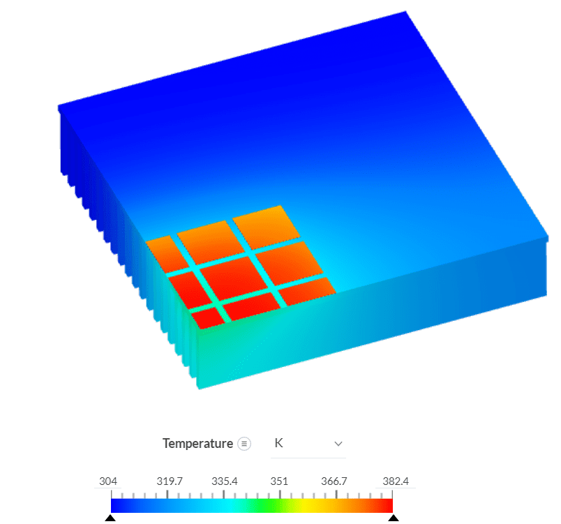
Figure 2: Temperature contour plot of an LED pack heat sink subjected to convective heat flux (see validation case below).
Markus LempkeComputational Designer at Siemens Energy
"Implicit modeling and direct simulations on implicit geometry is a real step change in speed and robustness of optimization workflows and necessary to unlock the real potential of additive manufacturing."
Professional
Request pricing
Antonio RadenićBattery System Engineer at Rimac Automobili
"Using SimScale in the early R&D stages of the product, we were able to fully leverage simulation capabilities into our product design process. This allowed us to quickly set up different cooling scenarios for our battery cells using SimScale's CHT module to efficiently analyze the impact of design changes on battery module performance."
"The design was complex, and using traditional simulation‑driven optimization to find the best‑performing configuration would have taken months. We now have an AI model that can generate a new optimized design in under an hour, and I have complete confidence in the results.”