Tutorial: Thermal Analysis of a Differential Casing

This article provides a step-by-step tutorial for the thermal analysis of a front differential casing. The objective of this simulation is to analyze the temperature distribution across the casing in operation mode.

This tutorial teaches how to:

• Set up and run a thermal simulation.
• Assign boundary conditions, material, and other models to the simulation.
• Mesh the geometry with the SimScale standard meshing algorithm.
• Explore the results using SimScale online post-processor.

The typical SimScale workflow will be followed:

1. Prepare the CAD model for the simulation.
2. Set up the simulation.
3. Set up the mesh.
4. Run the simulation.
5. Analyze the results.

1. Prepare the CAD Model and Select Analysis Type

To start, you can import a copy of the project into your workbench to follow along the steps by clicking the button below:

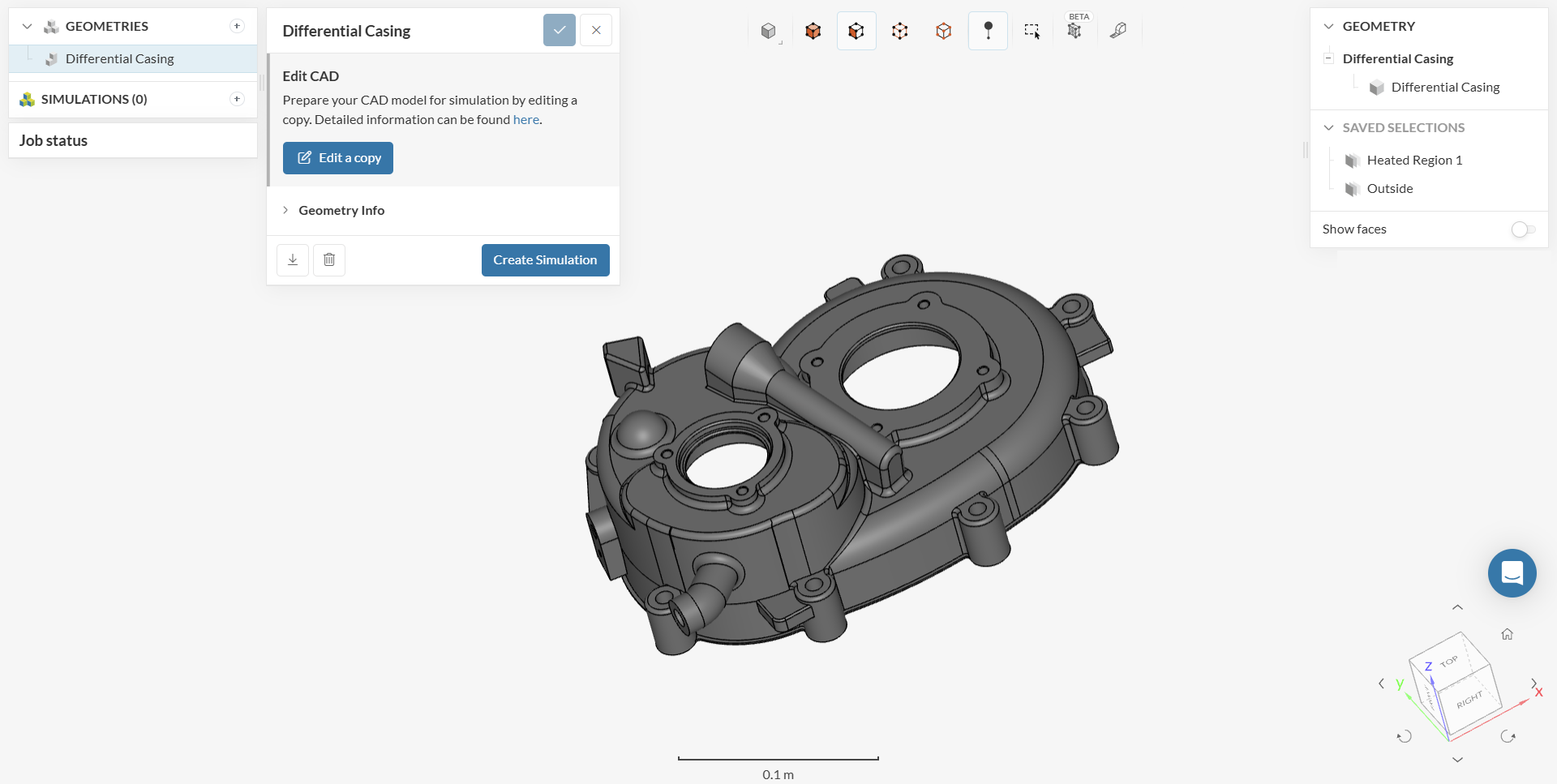
The following picture shows what should be visible after importing the tutorial project. You can find the geometry ‘Differential_Casing’ and the 3D model displayed. You can interact with the model as with any CAD program.

1.1 Create a Saved Selection

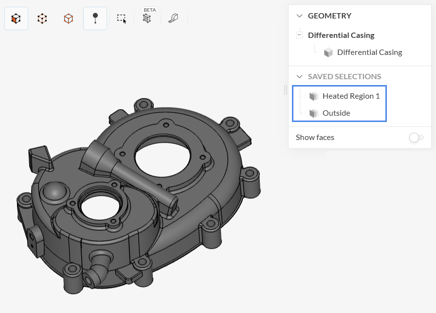
Especially interesting for our simulation is the creation of Saved Selections, which basically means that we can group faces together for later boundary condition assignment. The initial project already contains two saved selections, which can be found on the right-hand side panel:

We would like to create a third saved selection, this time for ‘Heated Region 2’, which will be used later for a boundary condition. The picture below shows how to create it:

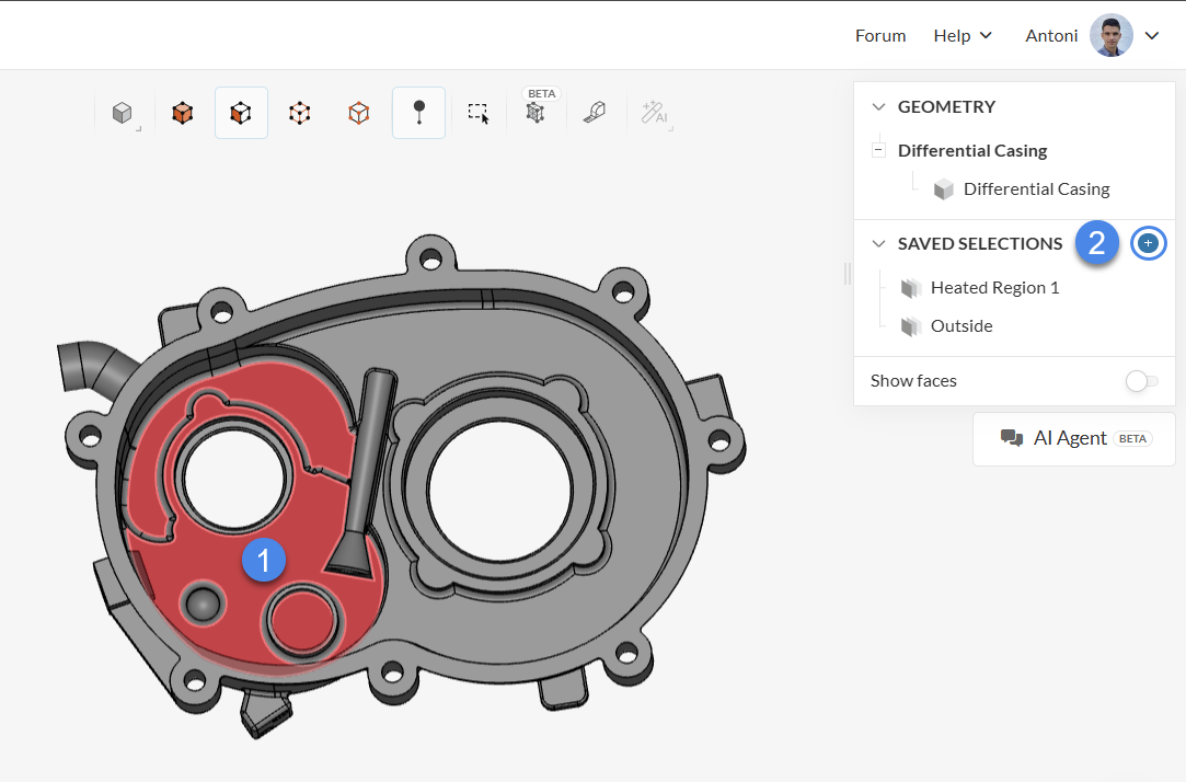
1. Select the corresponding set of faces as shown.
2. Click the ‘+’ icon at the right of Saved Selections in the right-hand side panel.

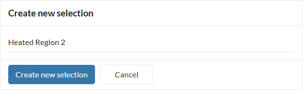
In the pop-up dialog that appears, name this selection ‘Heated Region 2’ and click the blue ‘Create new selection’ button.

1.2 Create a Heat Transfer Simulation

Now the simulation setup can be started. Follow these steps to create a new simulation:

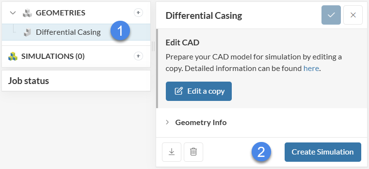
1. Select the ‘Differential_Casing‘ geometry element at the left panel.
2. Click on the blue ‘Create Simulation’ button in the pop-up window.

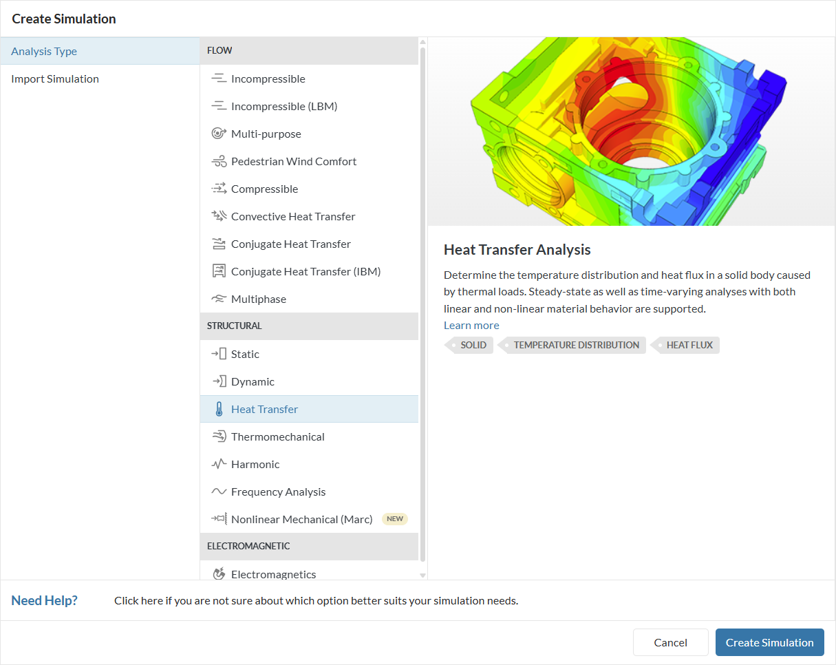
The simulation library window appears. Select the ‘Heat Transfer‘ analysis type and click the blue Create Simulation button as shown in the picture:

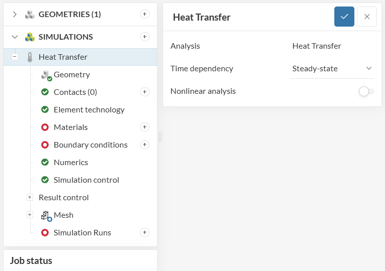
Now a new simulation tree will be automatically generated in the left panel with all the parameters and settings that are necessary to define to perform such an analysis. All parts that are completed are highlighted with a green check. Parameters that need to be specified have a red circle, while the blue circle indicates an optional setting that does not need to be filled out. You should see the interface as shown in Figure 8 below:

You can read more details about the heat transfer simulation type in our documentation page and the SimWiki page.

2. Setup the Simulation

2.1 Material Model

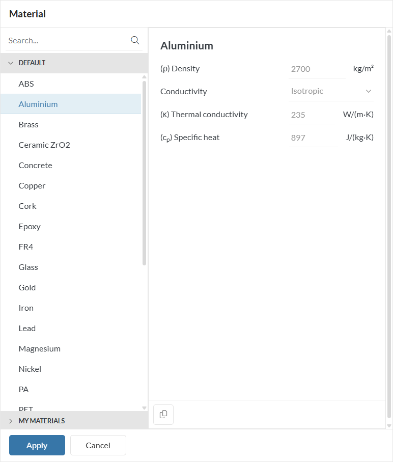
Next, add the material model from the ‘Material Library’. First, we start with clicking the ‘+’ button next to the Materials tree element at the left panel. This pops-up a ‘Material Library’ from which we select Aluminium and click on the blue ‘Apply’ button. This will then load the standard properties for Aluminium.

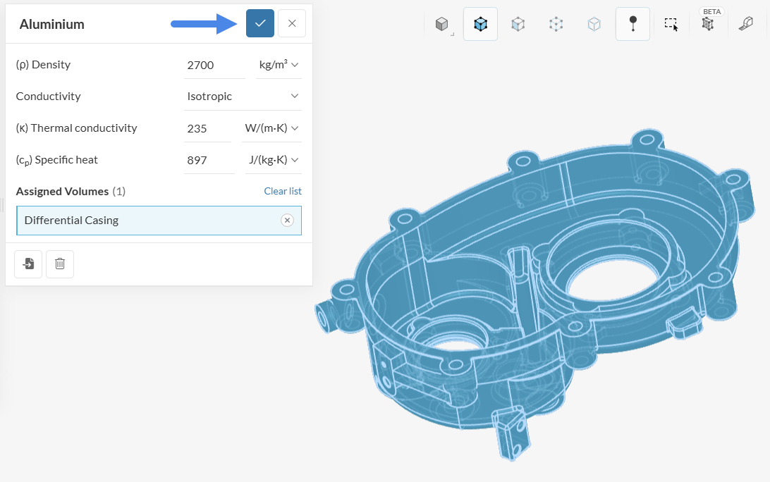
After hitting the apply button, our only body is automatically selected in the pop-up material properties window. Accept the selection with the blue check-mark button.

2.2 Boundary Conditions

Now, we come to define the boundary conditions. To create a boundary condition, click on the ‘+’ button option next to the ‘Boundary conditions‘ element at the left panel, and select the required boundary condition type from the drop-down menu, as shown in the figure.

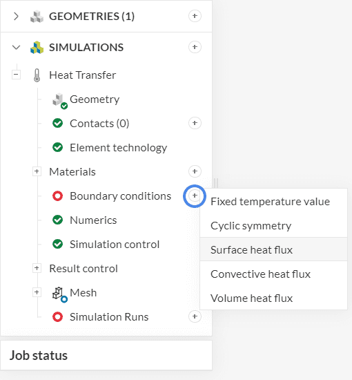
We can see that we can define either fixed temperature or heat flux boundary conditions. For our simulation, we’ll only need heat flux boundary conditions, since we will assign a specific heat load inside the casing and a convection condition on the outside.

A. Heated Region 1

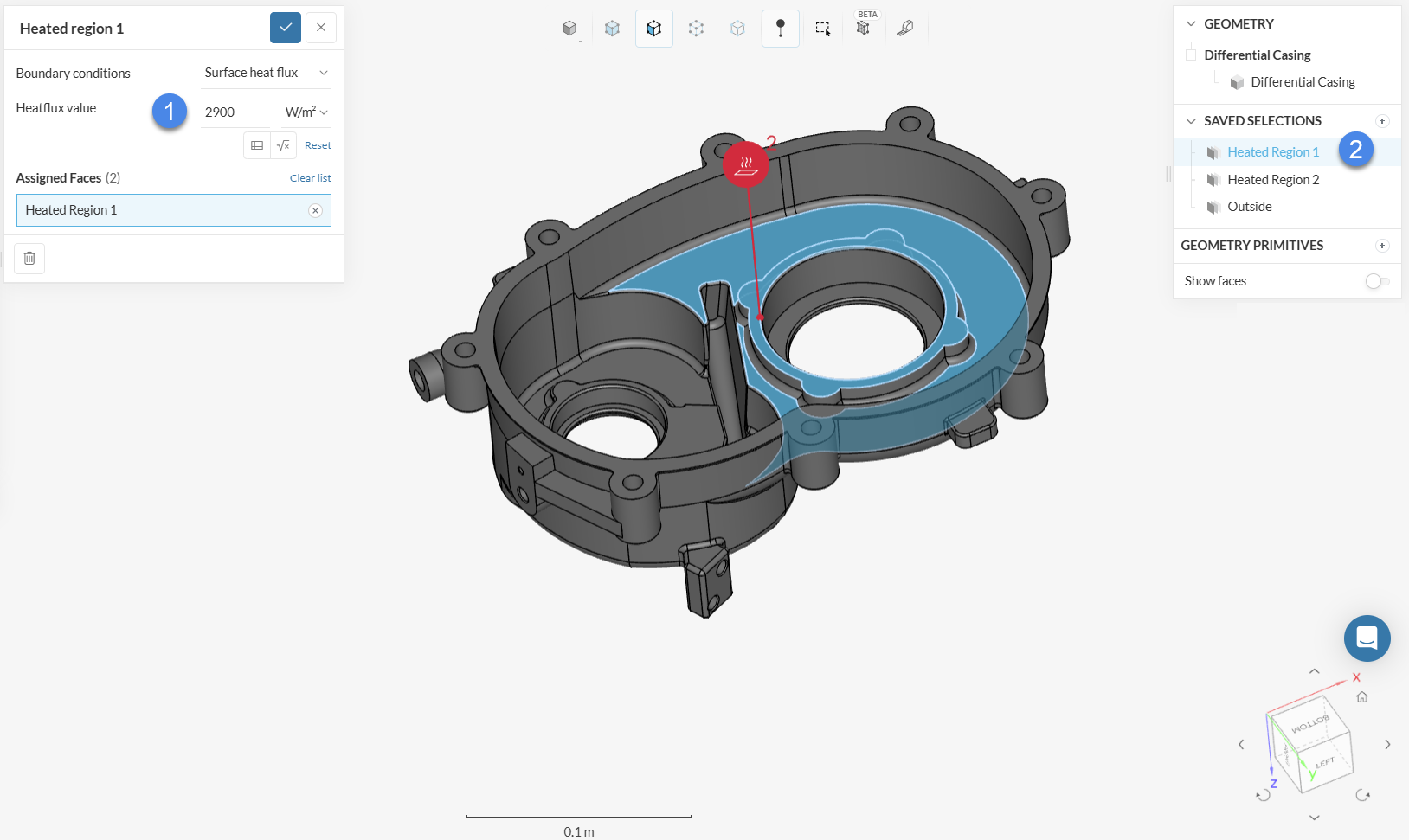
We will start with the first inner heat loss boundary condition for the Heated Region 1 saved selection. Select a ‘Surface heat flux’ boundary condition from the boundary conditions drop-down menu. Give a heat flux value of ‘2900’ \(W/m^2\), since this comes close to the thermal conditions we want to test in this simulation. Assign this to the Heated Region 1 saved selection If you would like, you can give an appropriate name to the boundary condition, such as Heated region 1.

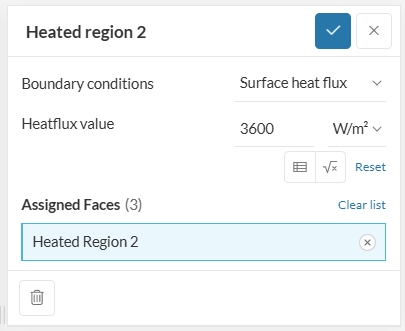
B. Heated Region 2

The second boundary condition is also a heat flux boundary condition of type Surface heat flux with a value of ‘3600’ W/m^2 assigned to the Heated Region 2 named selection.

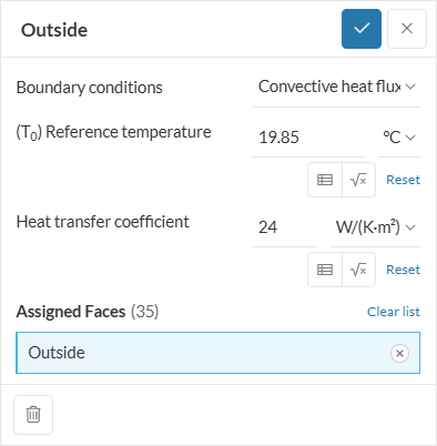
C. Outside Faces

The third boundary condition is a heat flux boundary condition of type Convective heat flux with a reference temperature of 19.85°C, and an h value of 24 W/m^2 K assigned to the named selection Outside. The value for the outside heat transfer coefficient for the convection boundary condition is taken from literature and is rather a rough assumption since this coefficient won’t be constant over the whole surface in reality.

These three boundary conditions are sufficient to simulate the thermal scenario we are interested in: Heat loss from the inside, and natural convection at the outside faces of the casing.

3. Mesh Setup

Select the mesh option and keep the default settings as shown in the figure below. You do not need to click the Generate button at this step, as the mesh will be computed as part of the simulation run.

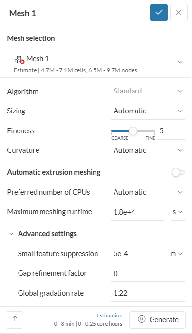
For this tutorial, a Fineness level of 5 is enough. As a rule of thumb, one should make sure that the resulting mesh does have more than one volume layer across the cross-section of the model.

Small feature suppresion value is also defined as 5e-4 in order to ignore features with sizes under the specified value. This will enhance better quality elements while reducing the unnecessary number of elements around small features which will have no effect on the solution.

4. Start the Simulation

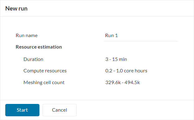
The last thing to do for running this simulation is to create a run. The new run is created by clicking on the ‘+’ button next to ‘Simulation Runs’:

In the pop-up window, you can give a meaningful name to the run, then click the blue ‘Start’ button to start the run.

The Job status box on the bottom of the simulation tree provides updates about the job status. Also, a Solver log is provided after a few seconds which shows the exact output of the actual computing algorithm. The simulation run should take a few minutes to be carried out. Once the simulation run is Finished we can Postprocess the results.

5. Post-Processing

Once the simulation run is finished, you can post-process the differential casing analysis results. To access the online post-processor on the platform you can use one of two methods:

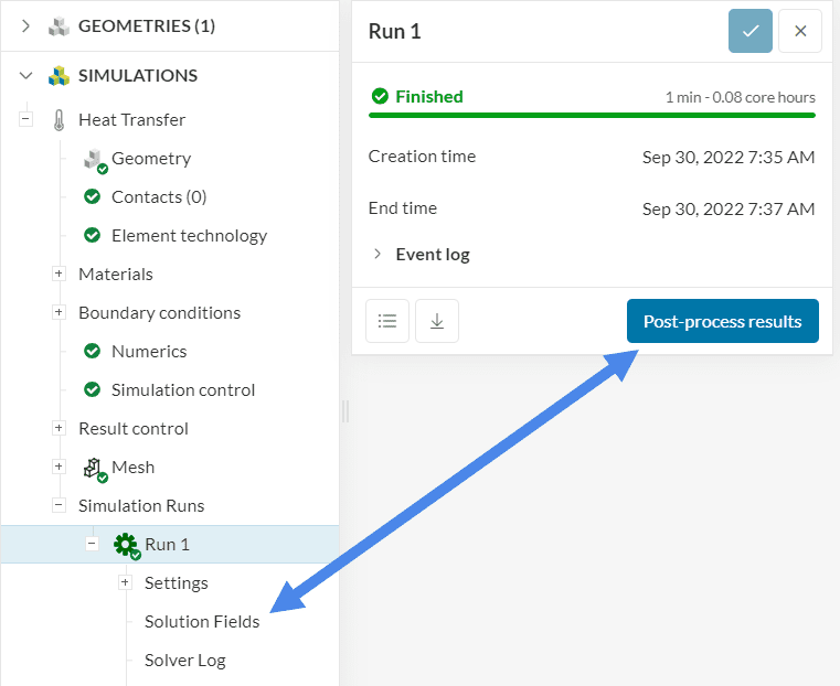
1. Select the ‘Solution Fields’ under the Run.
2. Click the ‘Post-Process’ button in the Run dialog.

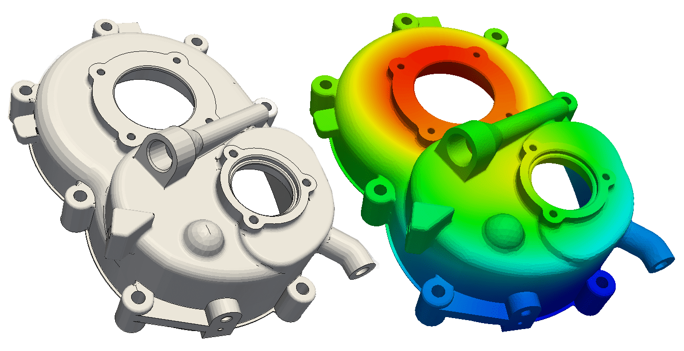
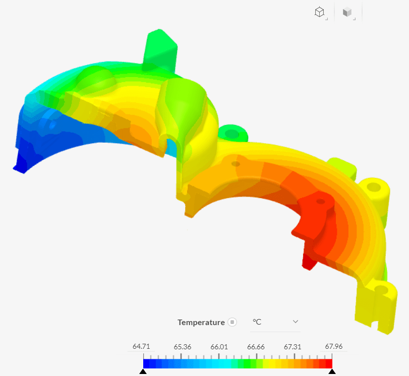
The default view state for the thermal simulation is to display the temperature distribution profile:

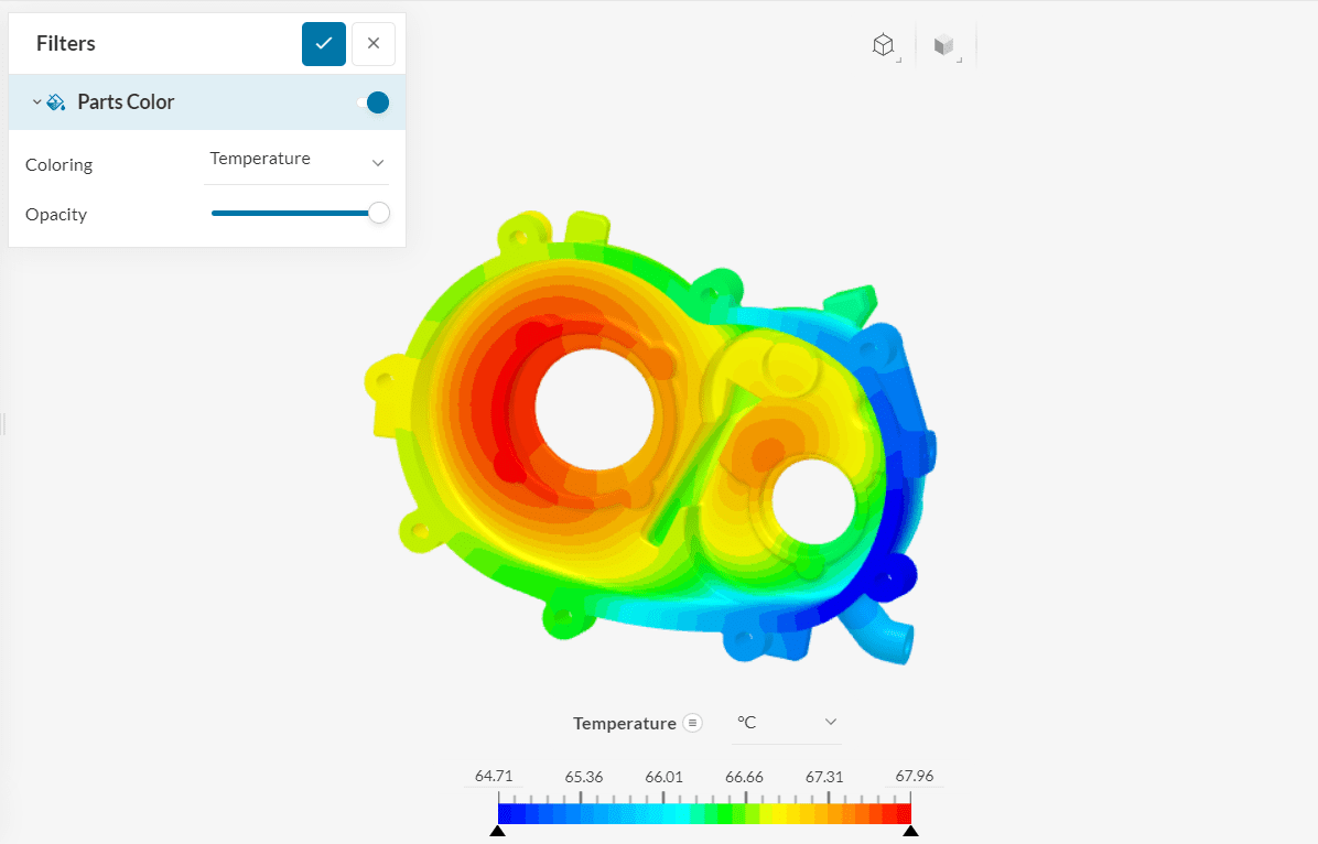
In this plot image, the blue color corresponds to the colder regions, and red corresponds to the hotter. The minimum temperature is found to be 64.71\(°C\), while the maximum is 67.96 \(°C\).

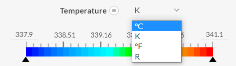
In case the temperature is displayed in Kelvins select the units drop-down menu to change to degree Celsius or other available temperature unit as desired.

We can visualize the temperature distribution inside the material by creating a Cutting Plane:

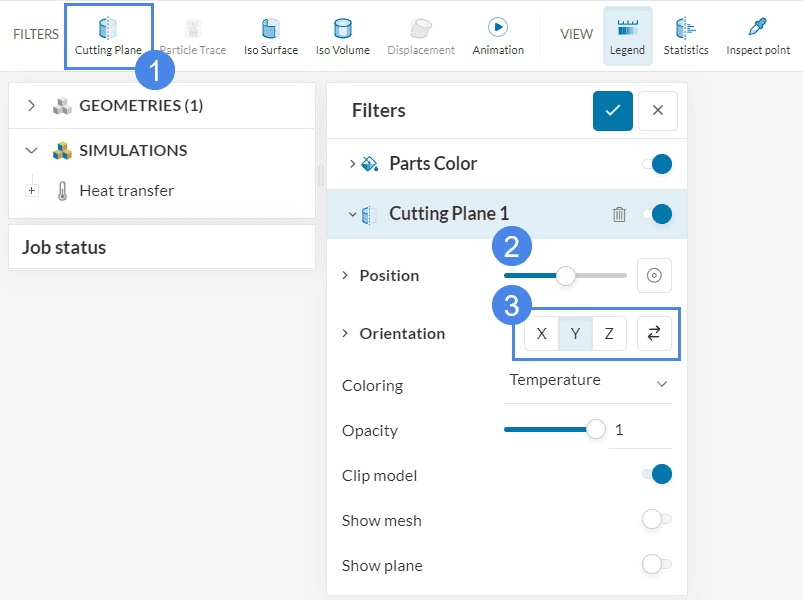
1. Select ‘Cutting Plane’ from the operations toolbar above.
2. Use the Position slider to move and locate the cutting plane across the geometry
3. Use the Orientation buttons to align the cutting plane normal to the global axes. In order to invert the portion of the geometry that is displayed, use the blue flip button.

The temperature gradient across the material can be appreciated in this plot. The hot and cold regions are consistent with the applied boundary conditions. Notice how, due to the thin walls, the gradient across the thickness of the material is barely noticeable.

Go ahead and try out for yourself what each one of the parameters does and what visualizations you can come up with. If you want to learn more about SimScale’s online post-processor, you can have a look at our post-processing guide.

Congratulations, you finished the differential casing tutorial!

Last updated: September 18th, 2023