Advanced Tutorial: Thermomechanical Analysis of an Engine Piston

This article provides a step-by-step tutorial for a thermomechanical analysis of an engine piston under maximum pressure and temperatures.

Overview

This tutorial teaches how to:

• Set up and run a thermomechanical analysis.
• Assign saved selections in SimScale.
• Assign boundary conditions, material, and other properties to the simulation.
• Mesh with the SimScale standard meshing algorithm.

We are following the typical SimScale workflow:

1. Prepare the CAD model for the simulation.
2. Set up the simulation.
3. Create the mesh.
4. Run the simulation and analyze the results.

1. Prepare the CAD model and select the analysis type

Firstly, you can click the button below and it will copy the tutorial project containing the geometry into your Workbench.

The following picture shows what should be visible after importing the tutorial project.

1.1 Create the Simulation

The first step of a simulation setup is to create a new simulation.

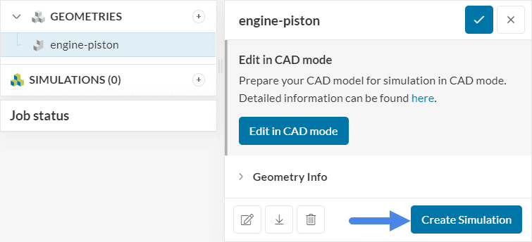
Hitting the ‘Create Simulation’ button leads to the following options:

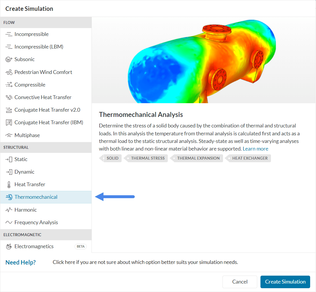
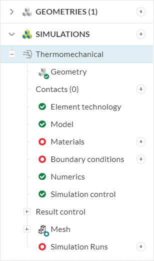
Choose ‘Thermomechanical’ as the analysis type and click the ‘Create Simulation’ button to confirm. After that, a simulation tree showing you all the necessary steps to set up your simulation will appear in your workbench.

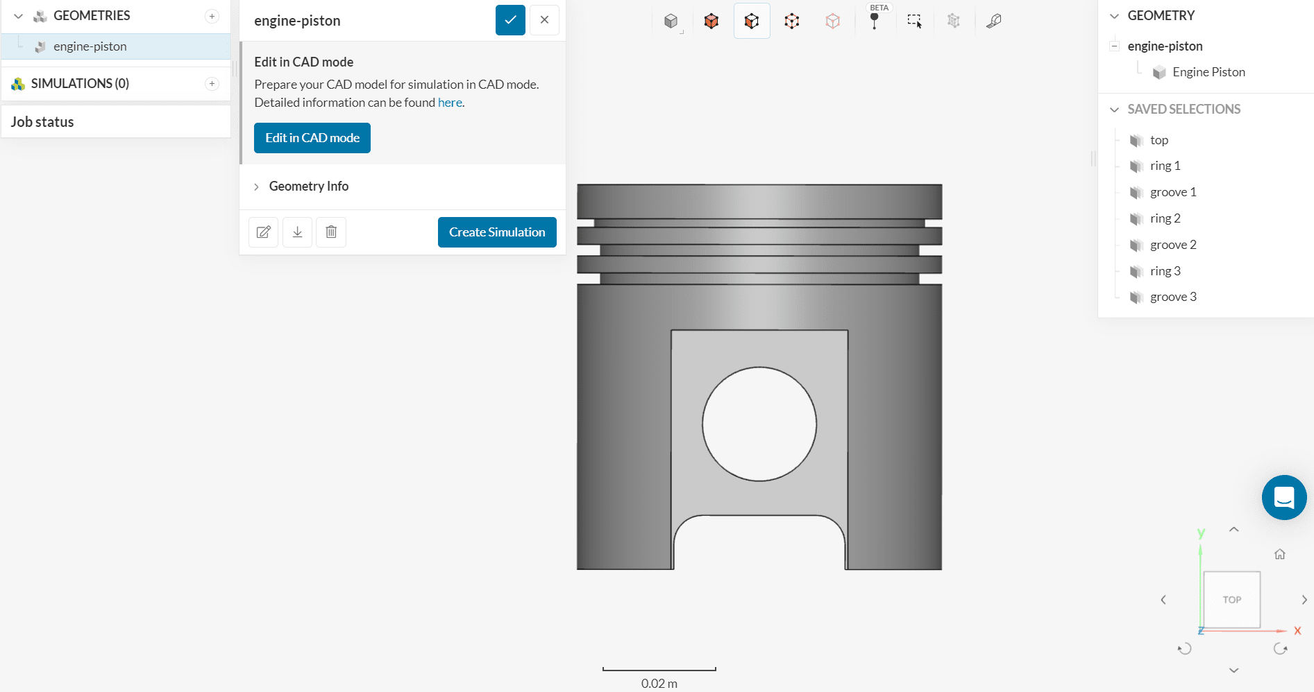
1.2 Create Saved Selections

Before setting up the simulation, we recommend creating saved selections. You can do this at any point of the simulation setup, however, it is easier to do it in the beginning.

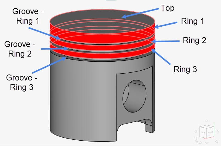
The selections for the top, the rings, and the ring grooves have already been created for you according to the following picture:

Now, you will only need to create the selection for the interior and the skirt of the piston, which is everything except the pre-created selections. Here are the steps:

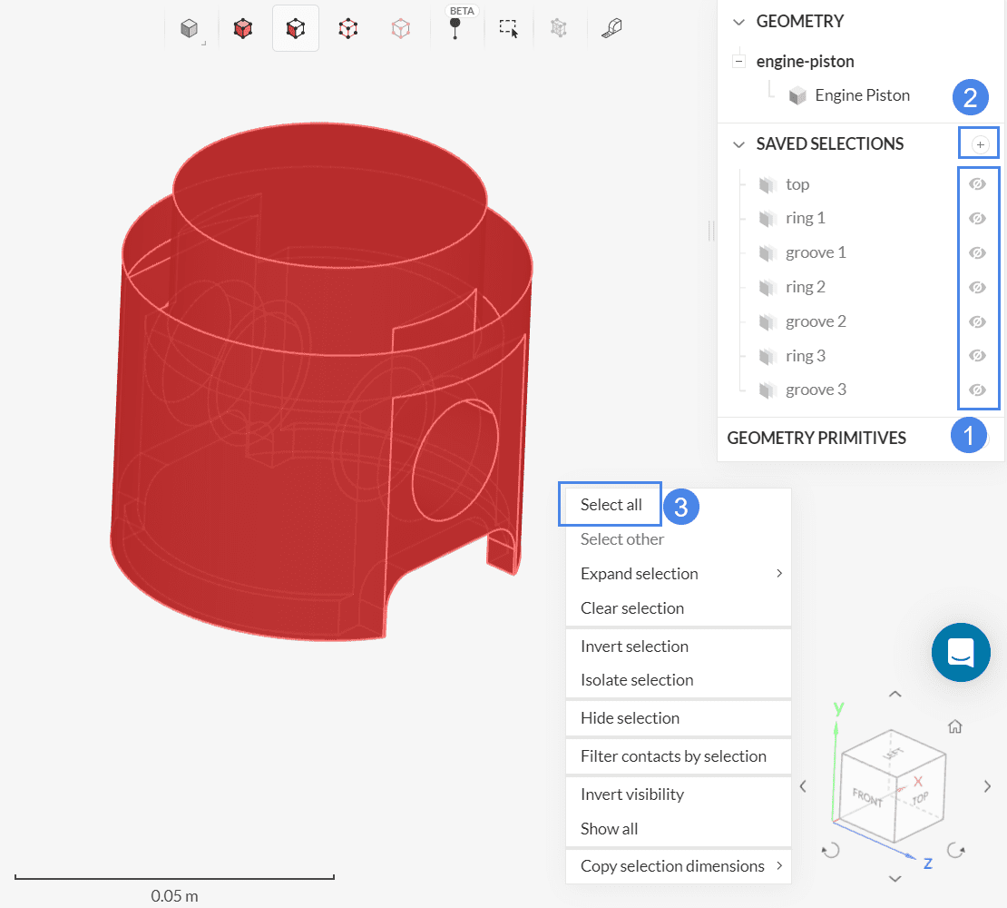
1. Hide all the existing saved selections
2. Right-click in the viewer and click on ‘Select all’
3. Hit the ‘+’ button next to Saved Selections and give a name to the new selection.

2. Assigning the Material and Boundary Conditions

In this section, we will define the physics of our model.

2.1 Model (Gravity)

Moving from the top to the bottom of the simulation tree, we have the Model tab, where we define the magnitude and direction of the gravity:

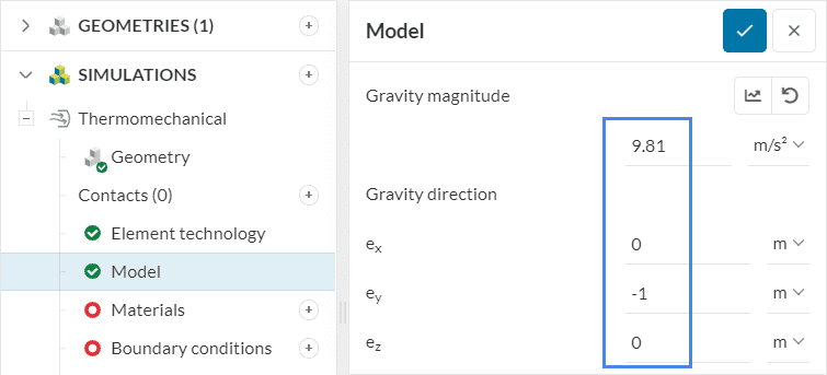
The magnitude of the gravity that we use is ‘9.81’ \(m^2/s\) in the direction ‘-1’ in \(e_y\).

2.2 Material

Afterward, we will define the material of our piston, which will be Aluminium. After clicking on the ‘+’ button next to Materials, the following list appears:

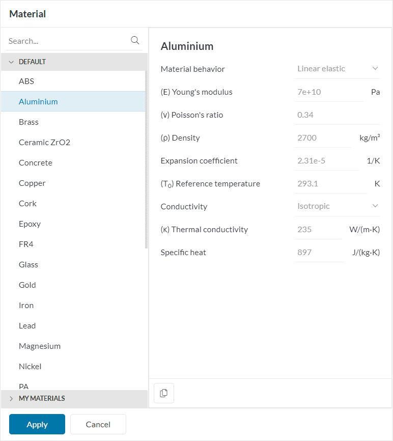
Choose ‘Aluminium’ from the list and confirm by pressing ‘Apply’. Since the CAD model from this tutorial contains a single volume, it will automatically receive the aluminium definition.

2.3 Assign the Boundary Conditions

A thermomechanical analysis will need two sets of boundary conditions: thermal and mechanical. In this section, we will define both sets of boundary conditions.

a. Thermal Boundary Conditions

We will use several Convective heat flux definitions as our thermal boundary conditions. You can therefore add a boundary condition by hitting the ‘+’ and selecting a ‘Convective heat flux’ boundary condition:

A convective heat flux boundary condition generates a heat flux based on the surface area, heat transfer coefficient, and temperature difference between the Reference temperature and the surface temperature.

The first convective heat flux boundary condition will have the following settings:

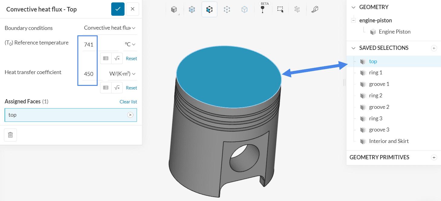
The \(T_0\) Reference temperature is 741 \(°C\), with a Heat transfer coefficient of 450 \(W/(K.m^2)\). This boundary condition is assigned to the ‘top’ saved selection. Alternatively, you can click directly on the top face in the viewer.

Follow the same procedure for the rows within the table below:

Saved Selection	Reference temperature [°C]	Heat transfer coefficient [W/(K*m^2)]
Ring 1	180	150
Groove – Ring 1	180	1000
Ring 2	160	150
Groove – Ring 2	160	400
Ring 3	140	150
Groove – Ring 3	140	400
Interior and skirt	120	650

b. Mechanical Boundary Conditions

Now it is time for the mechanical conditions, which will be three Pressure definitions (top and the first two rings) and two Remote displacements. At first, we will create a new boundary condition, this time choosing ‘Pressure’ from the list, and give it the following definition:

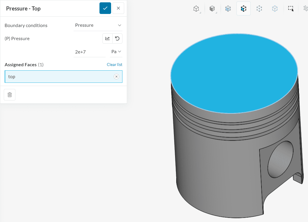
The first pressure boundary condition is assigned to the ‘top’ face of the piston, with a value of ‘2e7’ \(Pa\). The pressure boundary conditions for the other parts can be seen in the table below:

Saved Selection	Pressure [Pa]
Ring 1	1.4e8
Ring 2	4e6

Now, you can create a ‘Remote displacement’ boundary condition and give it the following definition:

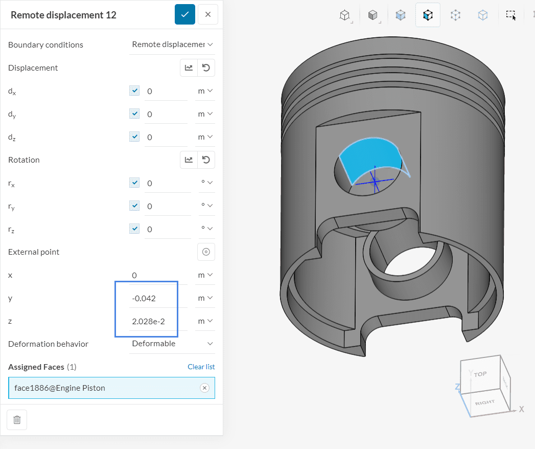
The first remote displacement is assigned to the top pin of the piston with the following coordinates for the External point:

• x: ‘0’ \(m\)
• y: ‘-0.042’ \(m\)
• z: ‘0.02028’ \(m\)

Following the same workflow, create a second ‘Remote displacement’ boundary condition, this time for the other side of the piston:

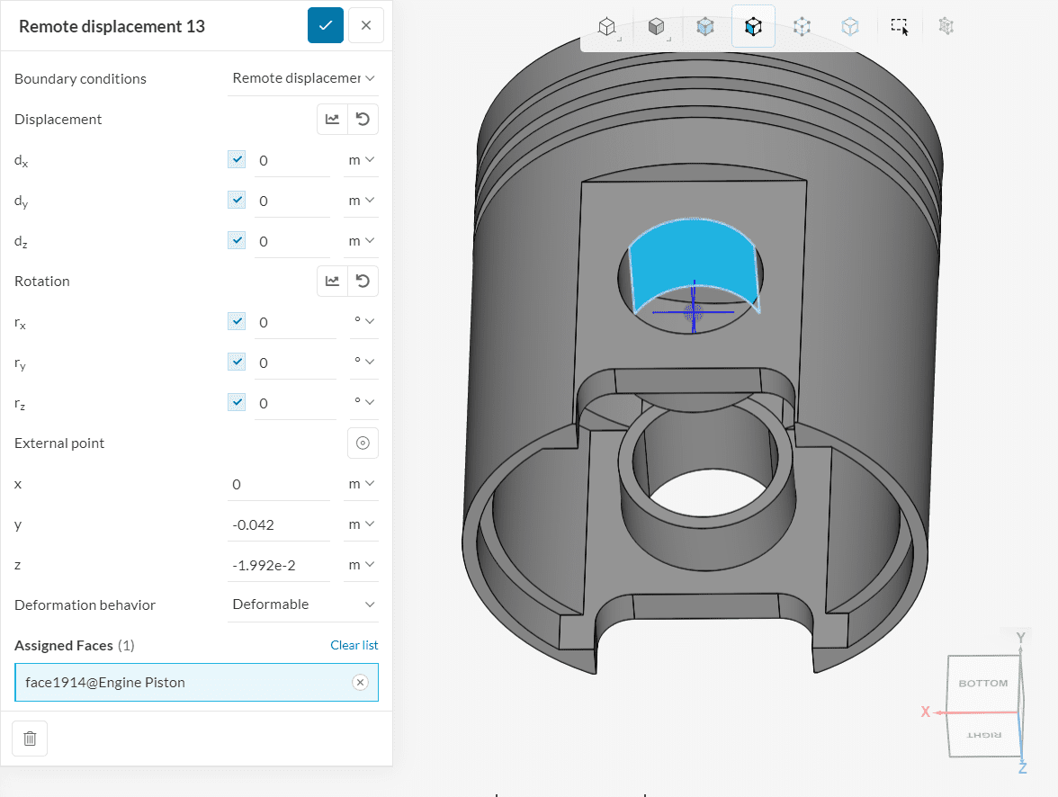
For the second remote displacement at the opposite side of the piston, please use the following coordinates for the External point:

• x: ‘0’ \(m\)
• y: ‘-0.042’ \(m\)
• z: ‘-0.01992’ \(m\)

Now all boundary conditions are assigned and we can proceed to create the mesh.

3. Mesh

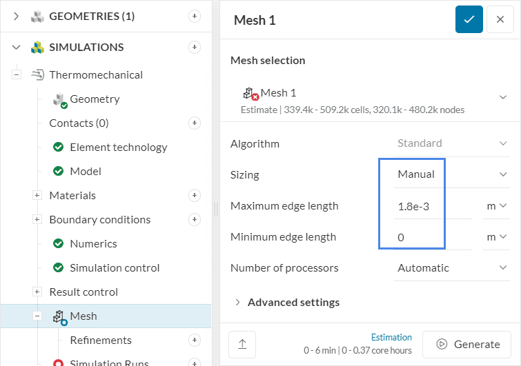
We will use the standard algorithm for our mesh, which is a good choice in general as it is quite automated and delivers good results for most geometries.

You will only need to change the Sizing to Manual and set our maximum edge length as 1.8e-3 \(m\). Make sure your settings look like the picture below:

When the mesh has been generated, it will look like this:

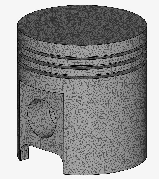
With default settings, a second-order mesh is created. Such meshes have additional nodes in between two connecting nodes, which helps to calculate deformations more accurately.

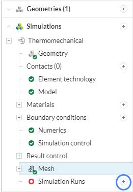
4. Start the Simulation

At this point, you can run your thermomechanical analysis for the engine piston by clicking on the ‘+’ button next to Simulation runs.

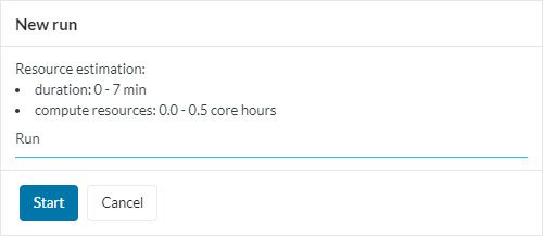
Moreover, you can change the name of your simulation to your liking and start the simulation by clicking ‘Start’

5. Post-Processing

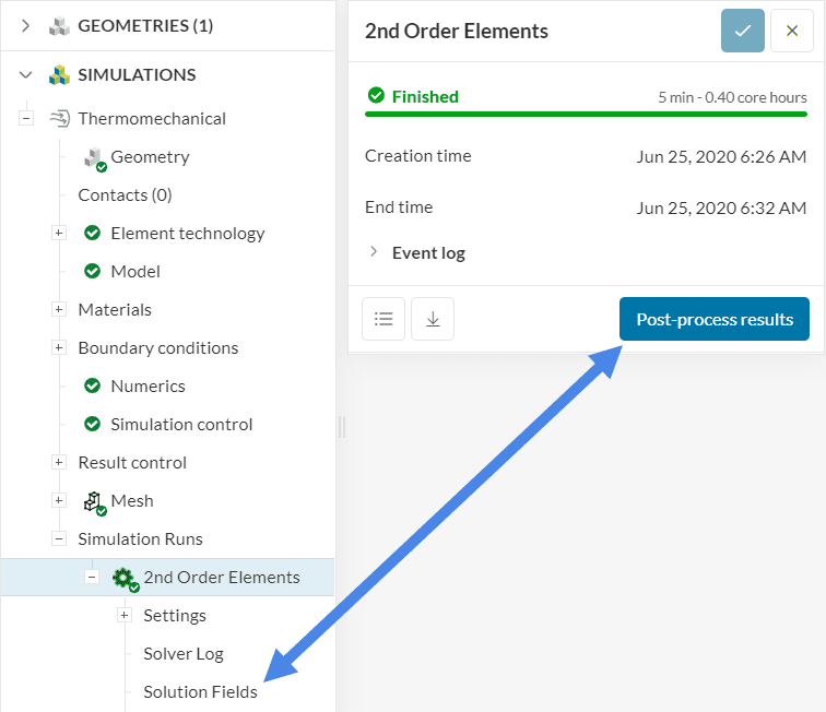
After the simulation has finished, you can access the simulation results by either clicking on ‘Solution Fields’ or by pressing ‘Post-process results’:

You can choose what results to visualize by going to the Filters panel:

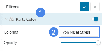
1. Expand the Parts Color section,
2. Select the desired field for Coloring.

5.1 Temperature

For example, we will start by plotting the Temperature field:

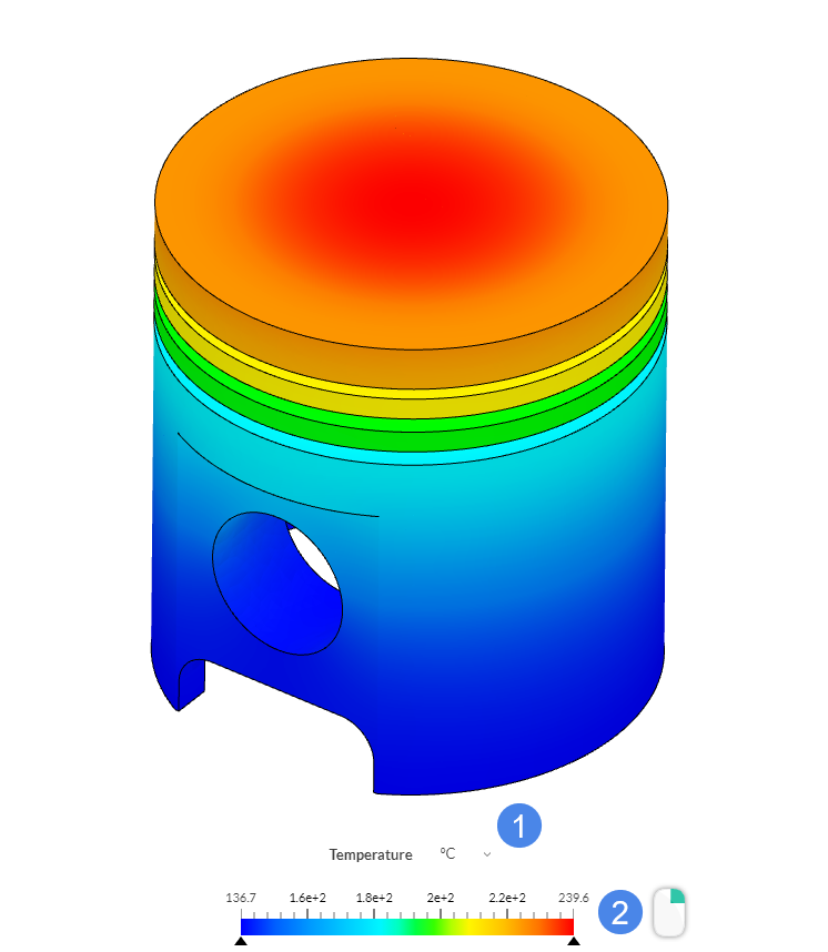
To achieve this visualization, we performed a couple of changes from the default state:

1. The temperature units were changed to \(°C\).
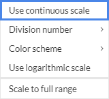
2. The ‘Use continuous scale’ in the context menu, which can be opened by right-clicking on the legend bar:

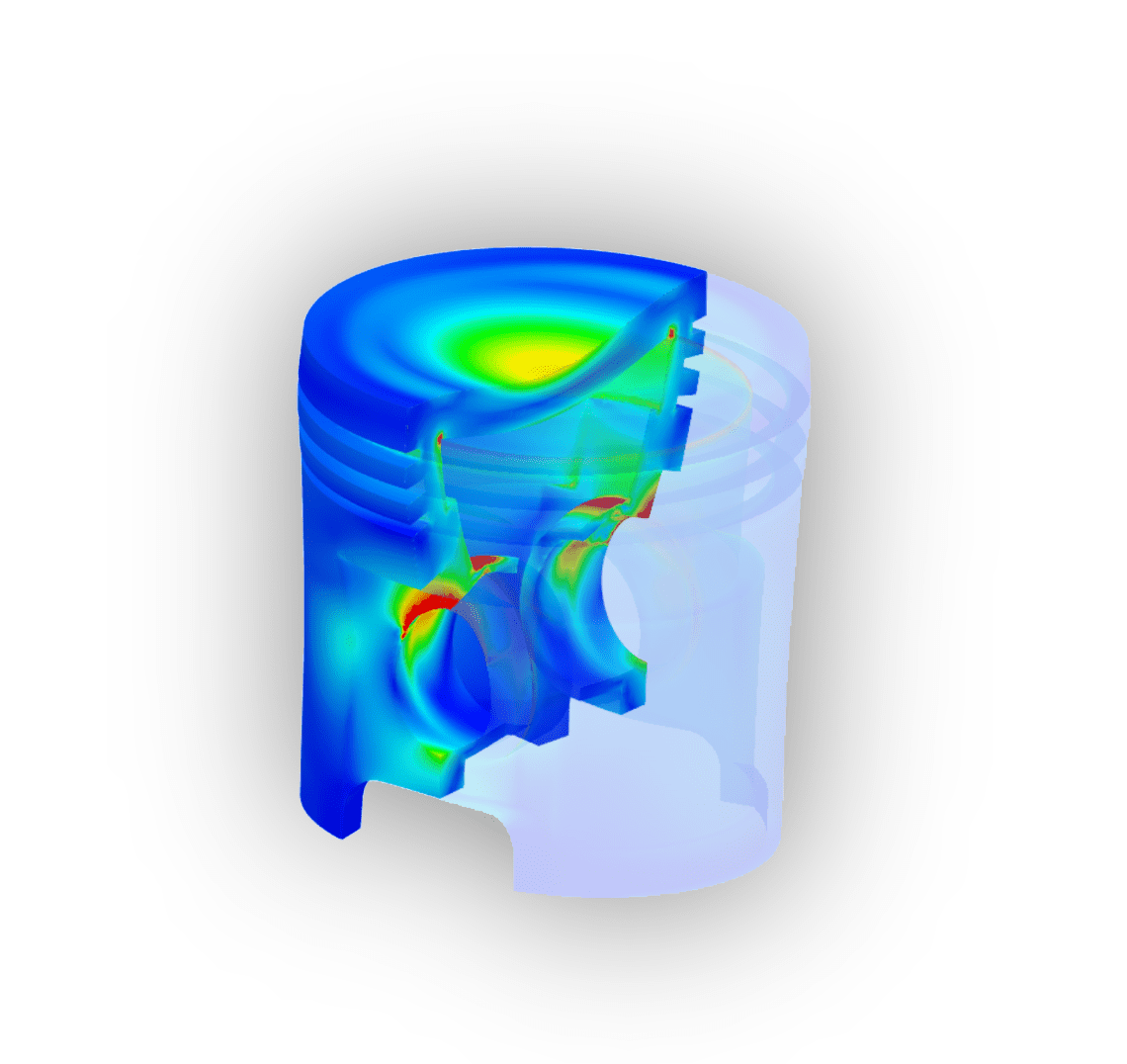
5.2 Von Mises Stress

We can also visualize the von Mises stress distribution with the same method:

1. Change the units to \(MPa\).
2. Use continuous scale.
3. Change the maximum value of the legend to ‘400’.

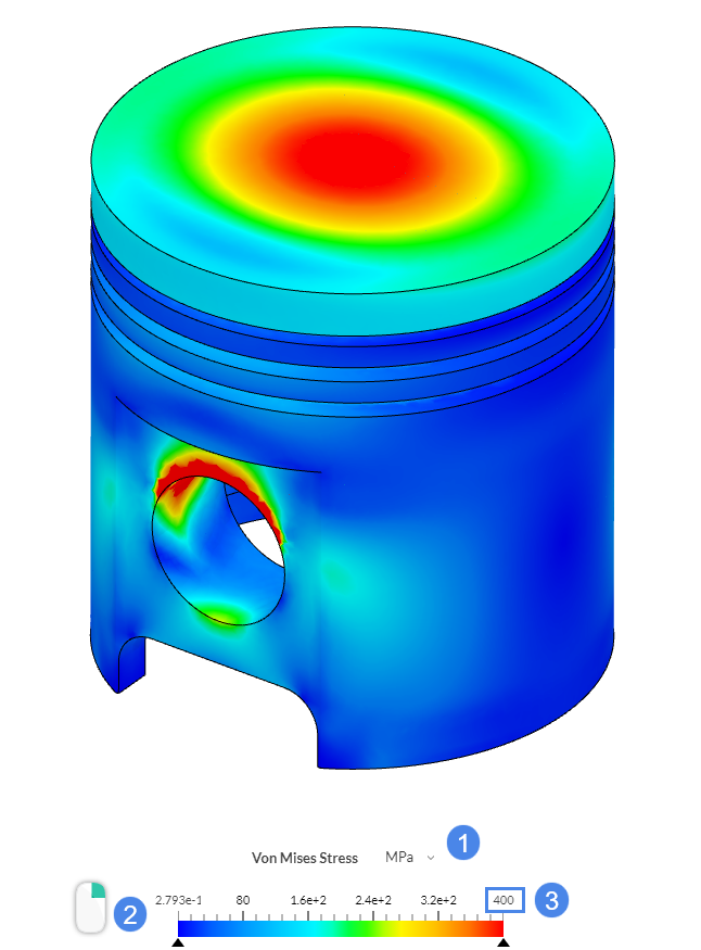
By lowering the maximum value of the color scale, we can create a threshold and find all the regions in the part where the stress exceeds this value. Those regions are colored in red in Figure 23 and are found in the support holes and the top face, where applied and reaction forces appear.

5.3 Deformation

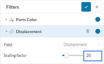
Finally, we want to visualize the deformation of the piston head. For this, make sure that the ‘Displacement’ option from the toolbar is active:

You might notice that the deformation is not apparent. This happens because the magnitude of the deformations is relatively small. To fix this, we changed the Scaling factor to 20:

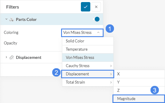
Also, to be able to find the magnitude of the deformations, you can switch the Coloring to ‘Displacement > Magnitude’:

Finally, we come up with the following plot:

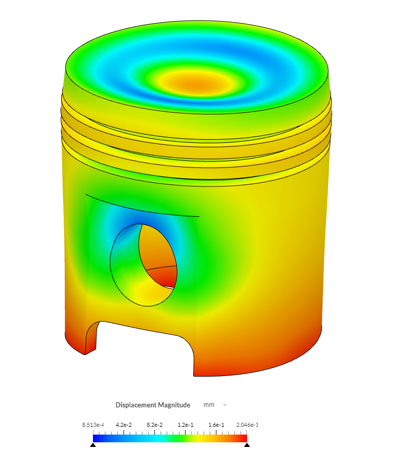
We can see how the piston head deforms due to the applied loads, boundary, and thermal conditions. The top face sinks, while the ring portion bulks out. We can also see the expansion at the bottom portion, which can be important for design purposes.

Congratulations! You finished the thermomechanical analysis of an engine piston tutorial!

Last updated: January 2nd, 2024